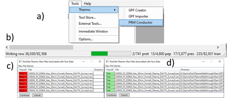
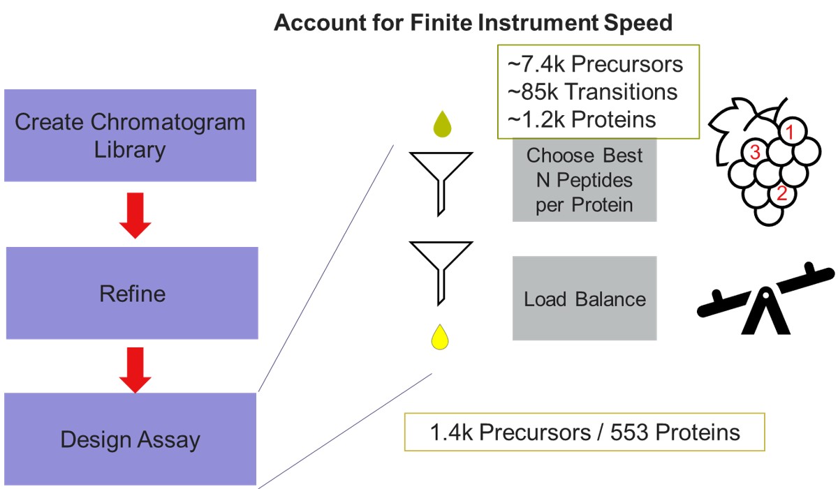
Once the results are imported into Skyline, the next step is to create a First-Draft version of the targeted assay using the PRM Conductor Skyline plugin. If you followed the steps in the tutorial, the Step 1. DIA GPF / gpf_results_importer.sky file should have opened after the import was finished, or you have the gpf_results_manual.sky version made. From one of these files, launch the PRM Conductor program (a), and Skyline’s bottom bar will report the progress of creating a Skyline custom report file that gets loaded by PRM Conductor (Figure b). Note that PRM Conductor depends on .raw files for some analysis, so it will look in obvious locations for the data files referenced in the Skyline file. If the raw files were not found, it will ask you to find the missing files. Once you double-click and use the file chooser to select them, the dialog will show a green “True” and you can continue. Even if the Skyline file used .mzml or another raw file format, just place the associated .raw files in a nearby folder and you can use the PRM Conductor.
Once loaded, the user interface in the figure below will be shown. There are 3 main parts to the user interface: a set of parameters on the left, a set of transition metric plots on the top right, and a set of precursor metric plots on the bottom right. We start with the Refine Targets parameters and the associated plots. Each of the text boxes has a corresponding graph on the right. The current value in the text box is a threshold value, and is displayed with the graph as a dashed, vertical line. The title of the plot reports how many of the transitions were filtered based on the current threshold. The blue distribution in the plot is for all the transitions in the report, while the red one is after all filters have been applied. Changing the parameter in the text box and pressing Enter will update the calculations in the plots on the right.
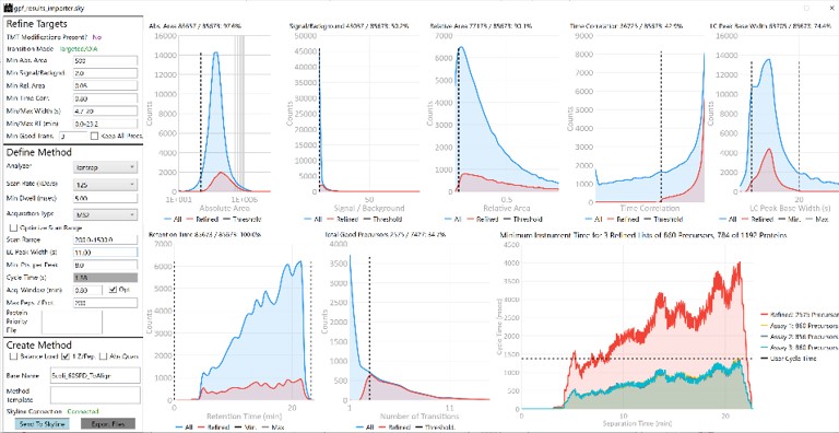
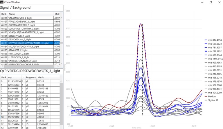
The first plot on the top is Absolute Area distribution. These are the Area values determined by Skyline for each transition. Note that these values are analyzer dependent, so a threshold used for Orbitrap discovery data may not be suitable for the Ion trap discovery data. The second plot is the Signal/Background distribution. These are the values of Area and Background as determined by Skyline for each transition. A traditional threshold for S/B is 3, however the user may wish to adjust to a different value. Highlighting the blue distribution and left-clicking will bring up a new window that gives the user an idea of what a particular S/B looks like in the Skyline transition data. For example, the figure below is a view of the plot after clicking the Signal / Background plot around 4. In the top left, all the transitions are in a grid, sorted by Signal / Background. On the bottom left is a grid showing all the transitions for the peptide corresponding to the selected transition on the top left grid. The graph on the right shows all the transitions for this peptide. The selected transition is highlighted in dashed lines. All transitions that currently meet the thresholds are colored blue, while the other transitions are colored grey. The red transition is the median transition trace.
The third plot on the top is the Relative Area distributions, that is, the area normalized to the largest transition for each precursor. The fourth plot is for the time correlation of each transition to the median transition for each precursor. The fifth plot on the top is for width of the transitions at the base, where a general rule is that outliers from this distribution may be poor quantitative markers, either because they are too narrow to characterize with the same acquisition period as wider peaks or are wide and potentially not reproducible. On the bottom row, the first plot is the retention time distributions. Precursors that are at the very beginning and very end may have the highest variability and could potentially be filtered out. The final transition filtering parameter is the Min Good Transitions text box. Many researchers prefer to set this value in the range of 3-5, to increase the confidence that a set of transitions is a unique signature for a peptide of interest. However, you could also click the Keep All Precs checkbox if you wanted to keep all the precursors, along with their best Min Good Transitions, which would potentially include some “bad” transitions. This is useful for cases with heavy standards where you don’t want to remove any of them. This is used in the Absolute Quantitation - PQ500 walkthrough.
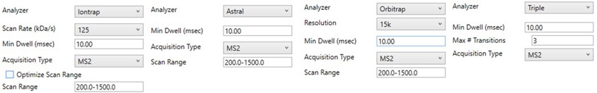
The next set of parameters on the left, in the Define Method box, control the acquisition parameters to be used in the targeted method. These parameters affect the speed of acquisition and the number of targets that can be scheduled in an analysis. The first parameter in the Define Method box is Analyzer. In this tutorial we are focused on Ion Trap analysis, but it is possible to make assays for other Analyzers. Selecting an Analyzer makes a specific set of parameters visible, which can change the characteristics of the analysis.
When any of these parameters are updated, the Scheduling graph on the bottom right will update. This graph shows the distribution of retention times for all Refined precursors in the red trace and the user’s chosen Cycle Time with the horizontal, dashed, black line. As we will see later, the user can choose to create a single assay that schedules as many precursors as will fit beneath that Cycle Time or may choose to create as many assays as necessary to acquire data for all refined precursors. The figure below shows views of the Scheduling graph in the single assay or “Load Balancing” mode, which we will talk more about below.
For peptide analysis, there is not much practical utility for the additional resolution afforded by the 66 kDa/s or 33 kDa/s over the “unit mass resolution” of the 125 kDa/s scan rate. Because for targeted methods we typically use the Dynamic Maximum Injection Time Mode in the instrument method file, the instrument allocates any additional time in the cycle to the targets according to their intensity. Therefore, the slower scan rates historically were useful mostly to guarantee a minimum amount of injection time per target, above the ~13 ms afforded by 125 kDa/s with the 200-1500 Th Scan Range, which can be useful for low concentration samples. With PRM Conductor, one can also set a minimum injection (or dwell time for QQQ users), which can accomplish the same thing. For peptides, we typically use the fixed 200-1500 Th scan range, because it guarantees this amount of injection time, gives a reasonable acquisition speed (~65 Hz), and the fragment ions in regions above and below this range are not essential to characterize most tryptic peptides.
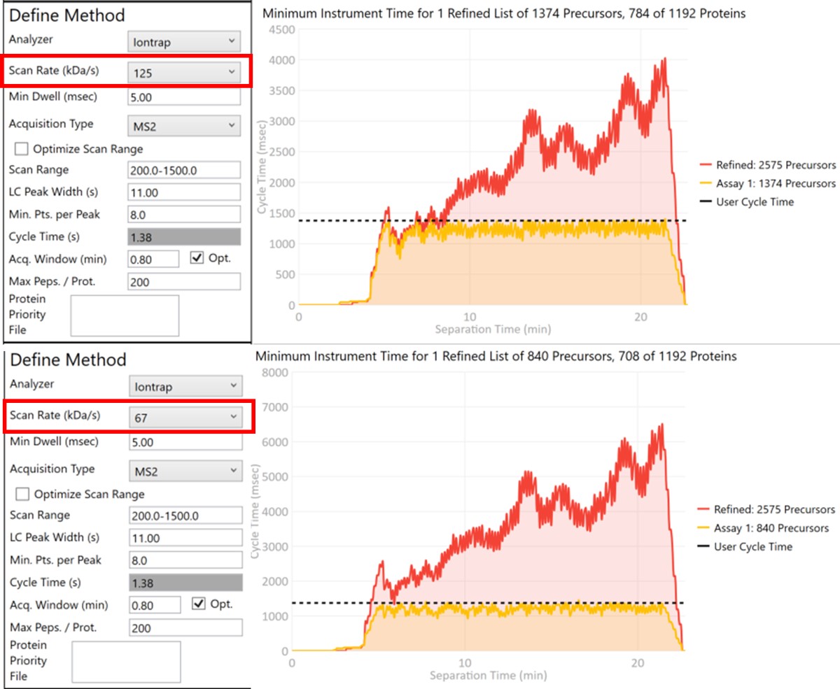
Let’s see what effect the Scan Rate has on the experiment. Changing the Scan Rate updates the estimation of how fast the instrument can acquire data. This is reflected in the Minimum Instrument Time plots, where in the top view, the Scan Rate is set to 125 kDa/s. An assay that would acquire data for all 2575 Refined Precursors would take 4 sec at the peak (at ~21 min), and 1374 precursors are able to be scheduled with the user-defined Cycle Time of 1.38 seconds. When the Scan Rate is set to 66 kDa/s (bottom part of the figure) the 2575 Refined Precursors would take 6.5 seconds of instrument time, and only 840 precursors can be scheduled with a Cycle Time of 1.38 seconds.
The user can change any of the parameters in this pane and visualize the effect on the assay. Of particular importance is the Acquisition Window. Stellar instruments are enabled with a new algorithm for real-time chromatogram alignment called Adaptive RT, which allows the instrument to adjust when targets are acquired to account for elution time drift. We find that an Acquisition Window setting of 0.75-1.00 minute usually results in good data, at least for the gradients we have typically used, in the range of 30 to 60 minutes. As LC peak width decreases for shorter gradients, we have successfully used narrower Acquisition Windows of 0.5 or even 0.3 minutes. Traditional tMS2 experiments, without real-time alignment, can sometimes require Acquisition Windows in the range of 3-5+ minutes. Adjusting this parameter allows to visualize the gain in number of targets afforded by narrower Acquisition Windows. For example, a 1 minute versus a 5 minute Acquisition Window allows to analyze more than 3x more targets (1172 versus 305). An additional feature related to Acquisition Window is the Opt check box. We have observed that the most variable part of many separations is at the beginning, which poses additional challenges for a real-time alignment algorithm because few if any compounds are eluting at the beginning. The Opt checkbox expands the Acquisition Windows somewhat, while still respecting the user’s Cycle Time requirement. The targets that are most improved by this algorithm are the early and late eluting targets; those where expanding their acquisition windows has little effect on the available injection time, but where alignment can be the trickiest.
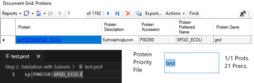
The last two parameters, which will be explored more below, are the Max Peptides per Protein, which helps to focus the analysis on just the highest quality peptides from each protein, and the Protein Priority File, which allows to create exceptions for particular proteins using their Skyline protein names.
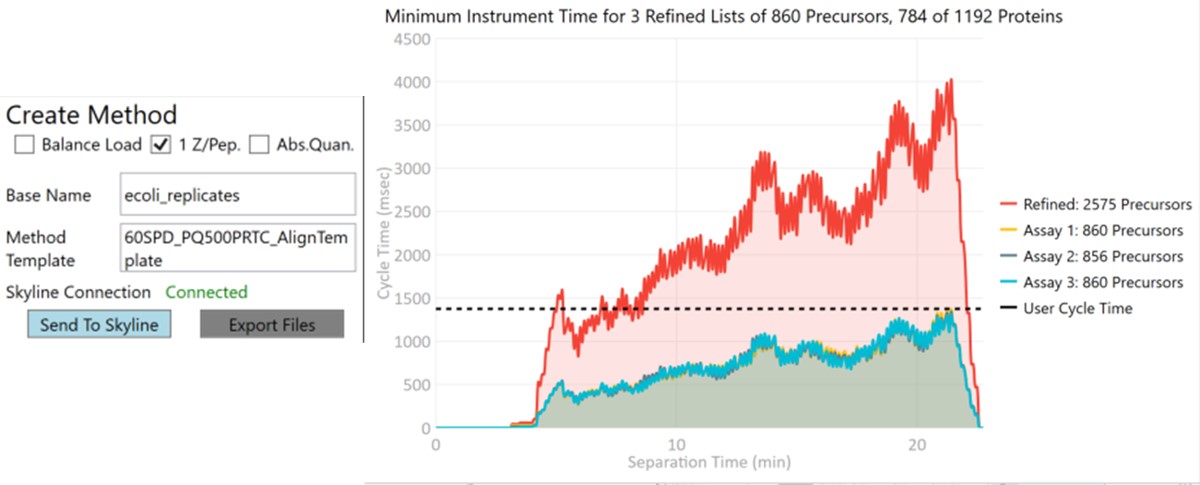
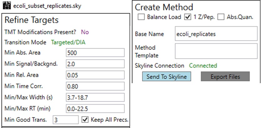
Now we will create multiple tMS2 methods for all the precursors that passed the filters and check to see which ones are stable and reproducible quantitative targets. To do this, uncheck the Balance Load button, which changes the Minimum Instrument Time plot so that all the Refined precursors are split into 3 assays, each of which require less acquisition time than the 1.38 second Cycle Time. Enter a base name for the file that will be created, otherwise the name “assay” will be used. Double-click the Method Template box and find the Step 2. Validation with Subsets/60SPD_PQ500PRTC_AlignTemplate.meth file. Then click the Export Files button.
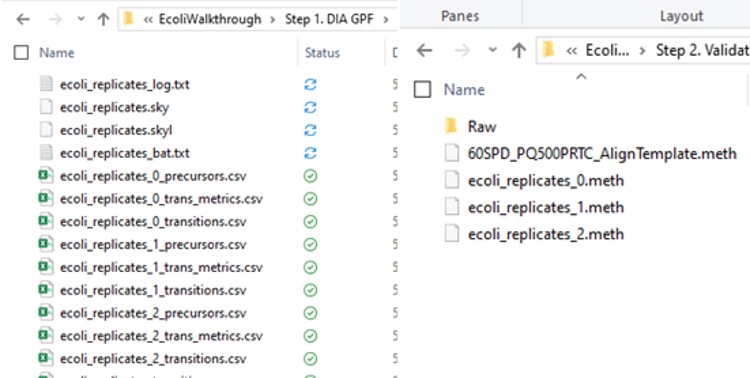
Some processing of the raw files will take place, as denoted by a progress bar, while the data files are aligned in time and a Adaptive RT reference file with the .rtbin extension is created. This processing only happens once, so if PRM Conductor is ever launched again for these raw files it won’t take as long to Export. The processing can take several minutes, depending on how many files are present and how long the gradient was. Method files will be created for each of the 3 assays in the same folder as the tempate method. A Skyline file will be created that is configured for tMS2 analysis with settings appropriate for the selected Analyzer. As a backup for the method and Skyline files, isolation and transition lists lists will be saved that are suitable for importing to the method editor or Skyline. The figure below is a view of the Step 1 folder showing some of the created files, and also the Step 2 folder showing the exported method files.
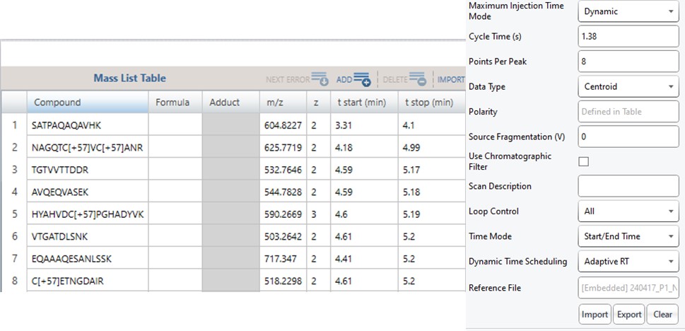
Note that because the 60SPD_PQ500PRTC_AlignTemplate.meth file had an Adaptive RT experiment and the tMSn method had Dynamic Time Scheduling set to Adaptive RT, the methods have embedded a .rtbin file to use for the real-time alignment. Notice too that the user’s Cycle Time and Points Per Peak were included, as well as the relevant precursors with their m/z, z, and scheduled acquisition times.
When exporting method files, a feature that can be useful is the Protein Priority File. There are two reasons to use this feature:
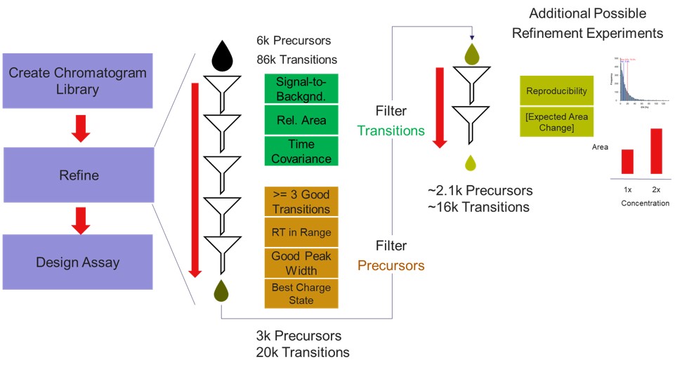
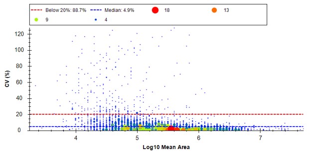
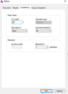
If the user desired, they could rely on just the results from the library to create a targeted assay. However, because a targeted assay may be used for many samples, we have found it worth the extra effort to further validate the set of precursors for reproducibility by performing several injections with each of the first-draft assays and filtering on a minimum coefficient of variation (CV) on the LC Peak Areas. In some more advanced scenarios where the assay is part of a multi-proteome mixture, one could perform injections for at least two concentrations of the proteome of interest, to ensure that the selected peptides change area with concentration appropriately, and thus belong to that proteome. In this tutorial we will demonstrate filtering performed on the LC peak area CV.
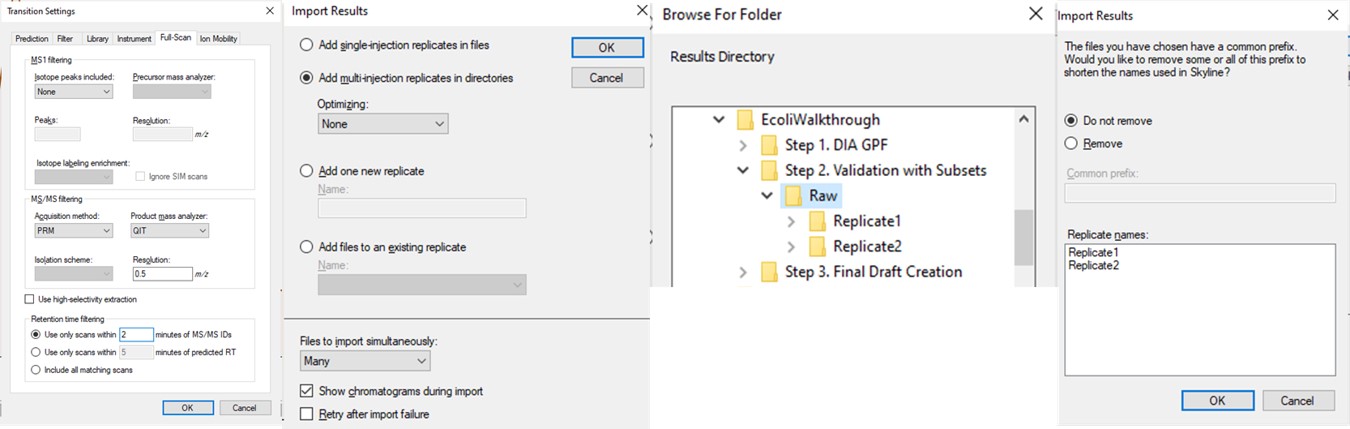
We performed 2 injections for the 3 first-draft assays. The program was in a slightly different state at the time, so the data collected don’t perfectly match the Skyline file created in the previous step, but they are very close. Normally we could just use the ecoli_replicates.sky file created in the last step for importing the results, but because of the different program state, we'll instead do a Save As on the Step 1. DIA GPF/gpf_results_importer.sky and save a new file, Step 2. Validation with Subsets/ecoli_subset_replicates.sky.
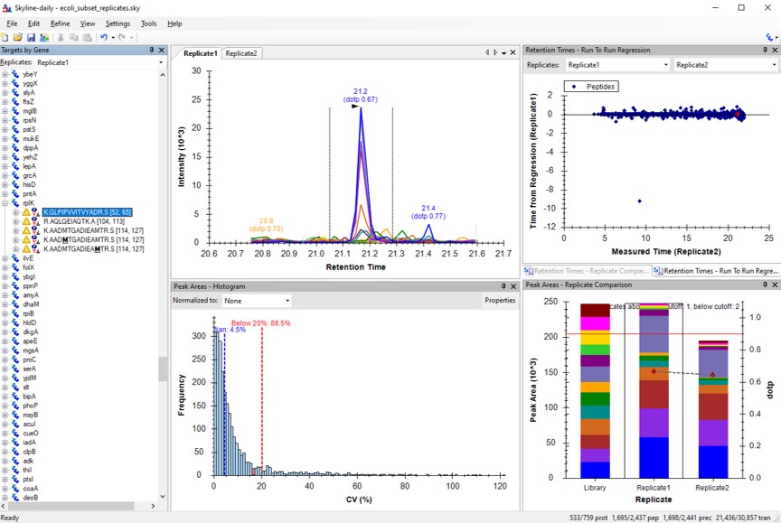
We have kind of a chicken-and-egg dilema now. As the .sky document currently has all of the up to 15 library transitions for each peptide, should we filter them first, and then filter the precursors by CV, or should we filter by CV and then filter the transitions? Here we opted to do the following to explore all the different options:
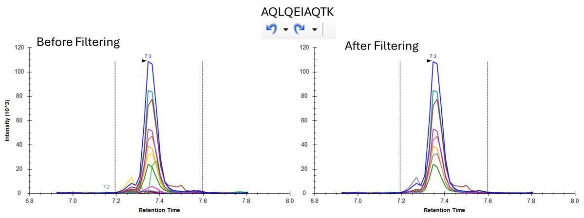
You can use the undo/redo buttons to see the effect that the filtering has had on the transitions. For example, in the figure below is shown the data for the AQLQEWIAQTK peptide before and after filtering.
Because we have a MS experiment in our method, the Total Ion Current normalization method is used, which can help normalize out experimental variation like autosampler loading amounts.
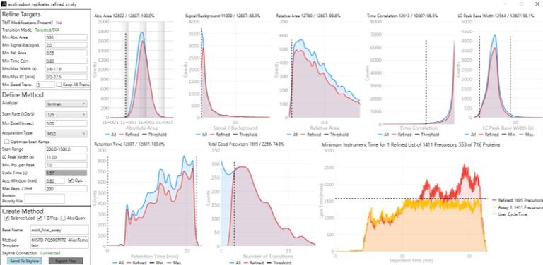
Now we will design the Final Draft assay. Our goal for this section is to ensure that the instrument can acquire quality data all the targets that are of interest. Here the experimenter can make certain concessions, such as, how many peptides per protein would give a usable result? Or am I willing to use 7 points across the peak instead of 10? We send the data to the PRM Conductor tool for analysis again using Tools/Thermo/PRM Conductor and get a View of the program like below. Compared to the earlier figure when PRM Conductor was run on the discovery results, these graphs are much different, because the precursors and transitions picked were already of such high quality. The percentage of transitions retained in the titles of each graph is close to 90% or greater. We set the LC Peak width to an even 11 seconds after hovering our mouse over the LC Peak Base Width graph to see the apex width, and set the Acquisition Window to 0.8 min.
This assay is what we would currently consider "normal", or conservative. There are 1411 precursors in a 24 minute method, which is about 3.5k precursors/hour. Had there been more precursors at earlier retention times, these settings would give about 5k precursors/hour. For fun, we have included HeLa results in the Step 1. DIA GPF\Processing\HeLaResults folder for those that wanted to explore what happens with a massive number of possible precursors.
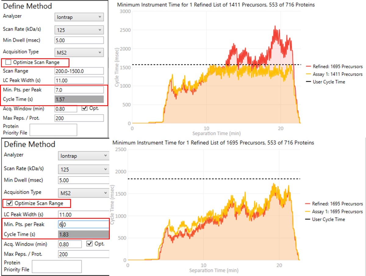
To realize the maximum throughput on Stellar MS, the user can select the Optimize Scan Range button, and could try using 6 points per peak, which is sometimes considered to be the Nyquist frequency for a Gaussian peak. We have successfully used such settings and observed little change in the results. The tradeoff being made with these settings is in the minimum amount of injection time per acquisition.
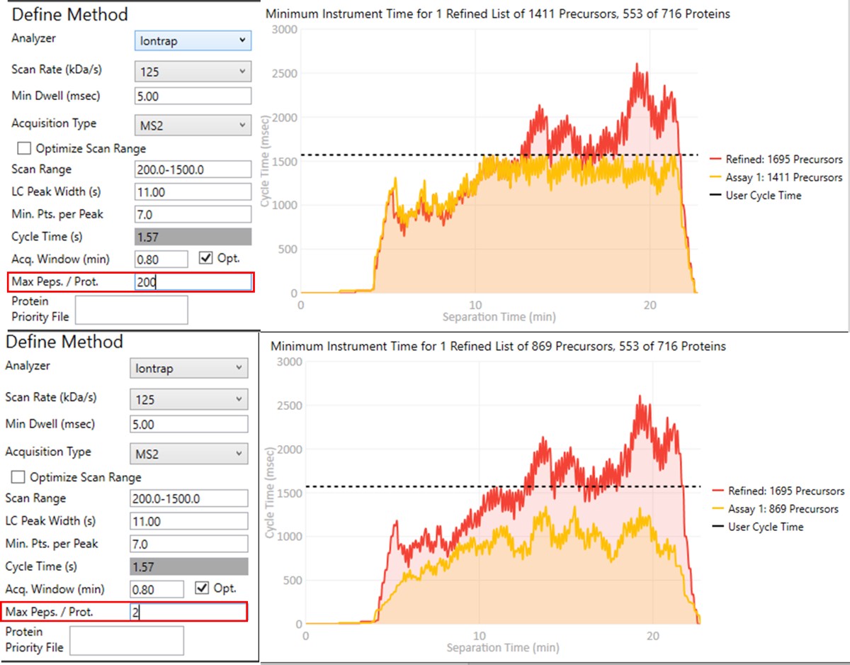
Notice that in above figures, the Balance Load check box is checked, and so the yellow Assay 1 trace in the Minimum Instrument Time plot is flattened up against the user Cycle Time. If the Max. Peps/Prot. value was reduced from 200 to 2, then the assay would contain only 869 precursors precursors, and there would be more space between the top of the Assay 1 trace and the horizontal cycle time line. Peptides are added from each protein in order of their quality from highest to lowest, as long as there is time at that point in the assay, and as long as the protein being considered has less than Max. Peps/Prot. peptides scheduled. It’s possible that an assay with fewer targets would have better quantitative performance, due to the longer available maximum injection times, and that could be of interest to the experimenter. In this example we leave the Max Peps./Prot. value at 200.
| Attached Files | ||
step2_1launch_prm_conductor.jpg step2_2prm_conductor_launch.jpg step2_3trans_window.jpg step2_4analyzer_options.jpg step2_5inst_time_plots.jpg step2_6multiassay.jpg step2_7exported_files.jpg step2_8created_method.jpg step2_9prot_priority.jpg step2_10workflow.jpg step2_11multiimport.jpg step2_12loaded_reps.jpg step2_13keep_all.jpg step2_14trans_filter.jpg step2_15_cv2d.jpg step2_16cv_filter.jpg step2_17loadbalance.jpg step2_18final_prm_conductor.jpg step2_19conservative_aggressive.jpg step2_20peps_per_prot.jpg