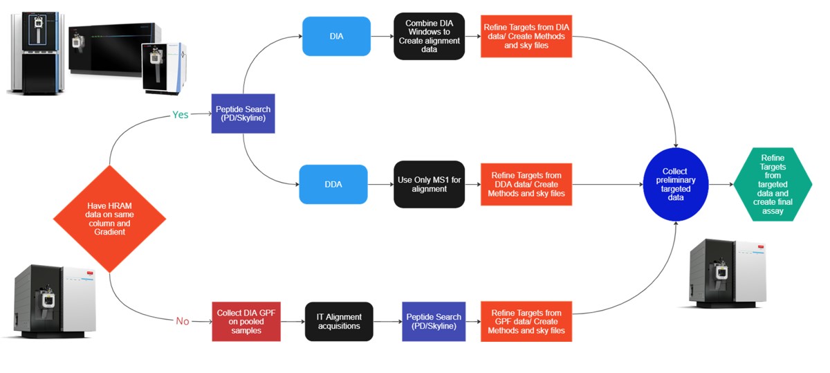
This tutorial will show you how to create a label-free targeted assay from discovery results. As shown in the figure below, there are two main routes to creating this kind of assay, to main difference being whether the discovery data comes from a high resolution accurate mass instrument like Astral, Exploris, or a Tribrid, or whether the discovery data comes from a Stellar. Once we have the discovery results in Skyline, the steps are largely the same. In this tutorial we'll look at an assay created from Stellar MS gas phase fractionation results.
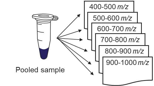
Our recommended technique for creating targeted assays starts with acquiring a set of narrow isolation window DIA data on a pooled or characteristic sample, creating what the MacCoss lab has termed a “chromatogram library”. This technique allows for a deep characterization of the detectable peptides in the sample, and the resulting data can be used to create a Skyline transition list of high quality targets. As outlined in in the figure below, generation of the library typically involves several (~6) LC injections, where each injection is focused on the analysis of a small region of precursor mass-to-charge. This technique has also been called “gas-phase fractionation” (GPF) to contrast with the traditional technique of off-line fraction collection and analysis. The GPF experiment should be performed with the same LC gradient as the final targeted assay, which allows us to use the library data for real-time retention time alignment during later tMS2 experiments.
Assuming that a pooled sample is available for analysis, the first step is to create a template instrument method file (.meth). Open the Instrument Setup program from Xcalibur, or the Standalone Method Editor (no LC drivers) if using a Workstation installation.
C:\Program Files\Thermo Scientific\Instruments\TNG\Thorium\1.0\System\Programs\TNGMethodEditor.exe
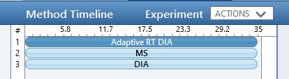
Use the method editor to open the file at Step 1. DIA GPF/60SPD_DIA_1Th_GPF.meth. This method includes 3 experiments:
Assuming that the user has configured their LC driver with the Instrument Configuration tool, the LC driver options would appear as a tab in the pane on the left-hand side of the method, where the user has to design the length and type of gradient program to be used. Of course, the choice of gradient length is of great importance as it determines the number of compounds that can be analyzed and the experimental throughput. A general rule of thumb is that Stellar can analyze on the order of 5000 peptides in an hour gradient, where this number depends on how the peptide retention times are distributed and other factors and settings that will be explored later in the tutorial. The user will need to make sure that the MS part of the experiment has the same Method and Experiment Durations as the LC gradient.
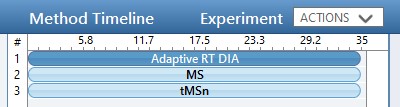
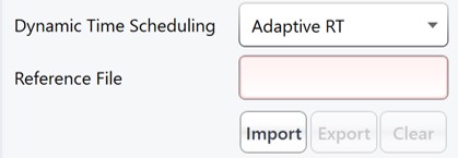
While we are making methods, we should create a tMS2 method template with the same LC parameters as the library method file. One can start with Step 1. DIA GPF/60SPD_tMS2_Template.meth. This method has the same first two experiments as the GPF template, and the 3rd experiment been replaced with a tMSn experiment. Our software tool will later fill in the targeted table information in a new version of this file, as well as update the LC peak width and cycle time parameters and embed the reference data for the Adaptive RT.
One thing to note about the targeted template is that the Dynamic Time Scheduling is set to Adaptive RT. When we save the method, a message tells us that the file is invalid because no reference file has been specified. This is okay, because PRM Conductor will fill in this information for us later.
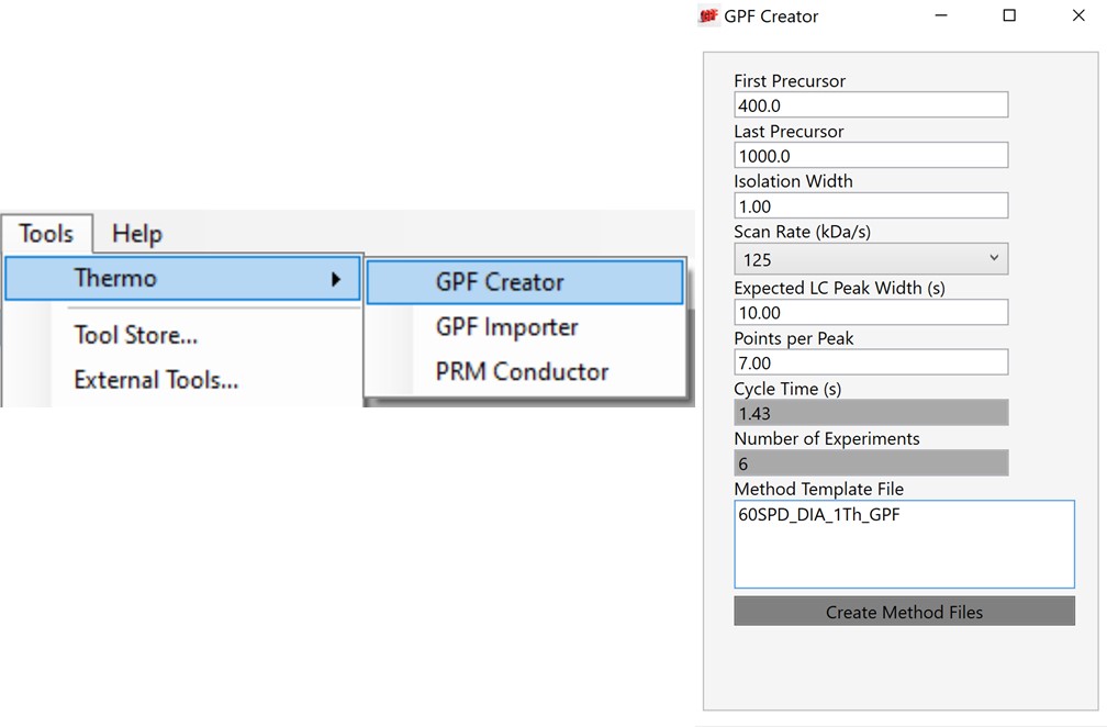
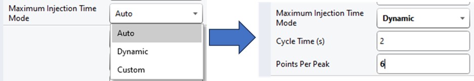
Once the GPF method template file is created and saved, the user should select that file with the GPF Creator tool. The tool will create a set of new methods based on this template, one for each precursor mass-to-charge region. The number of method files to be created depends on the settings in the user interface. The default precursor range for the tool is 400 to 1000 Th, as most tryptic peptides have a mass-to-charge ratio in this range. We recommend, for Stellar, to use an isolation width of 1 Th, which allows the DIA data to be searched even with traditional peptide search tools like SEQUEST and allows for a good determination of which transitions will be interference free in the tMS2 experiment. However some users have used 2 Th windows, in order to user slower scan rates and/or more injection time per scan without having to acquire 2x as many GP fractions. If the experiment Maximum Injection Time Mode is set to Auto, then the maximum injection time is the largest value that does not slow down acquisition, which depends on the Scan Rate. For this simple tool, we assume a scan range of 200-1500 Th. The largest amount of injection time and the slowest acquisition rate is afforded by the 33 kDa/s scan rate, and the smallest amount of injection time and the fastest scan rate is afforded by the 200 kDa/s scan rate.
For most applications, we prefer to use 67 or 125 kDa/s and set the Maximum Injection Time Mode to Dynamic as in the figure below, which lets the maximum injection time scale with the time available in the cycle.
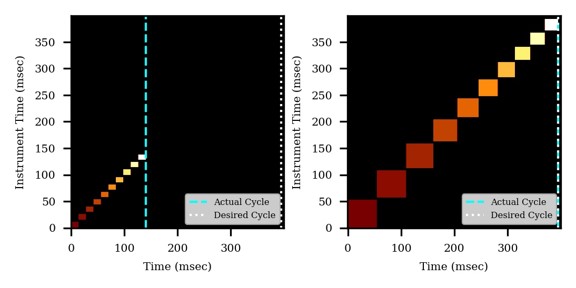
If the Cycle Time is set to 2 seconds and the cycles take less than 2 seconds, then the remaining time in the cycle is distributed to the acquisitions inversely proportionally to the intensity of the precursors, ex. less intense precursors get more injection time. In this figure, the left panel shows a hypothetical situation at the start of a cycle. We calculate the minimum amount of time that each of the acquisitions needs, and sum this to get the blue, vertical, dashed line. The remaining time in the cycle is the white, vertical, dotted line. Each acquisition is colored, with the most intense precursors colored white, based on previous data. In the right panel, the amount of time the acquisitions actually take is displayed, where the less intense precursors were given more injection time.
The expected peak width in GPF Creator is the LC peak width at the base in seconds. This value can be determined by checking a few peaks in a quality control (QC) experiment, for example an injection of the Pierce Retention Time Calibration standard. The LC peak width combined with the desired number of sampling points across the peak width, the isolation width, and the Scan Rate determines the number of LC injections needed to create the library.
Once the parameters are set, the user selects the Create Method Files button, which will create the instrument method files needed for the library. The user can create a sequence in Xcalibur and run these methods along with any blanks and QC’s that they want. We have collected data for a mix of 200 ng/ul E. coli with 200 ng/ul HeLa, and placed the resulting raw files in Step 1. DIA GPF\Raw.
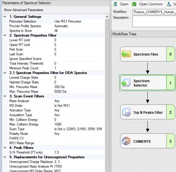
The next step is to search the data to find candidate peptide targets. Ion trap DIA data with 1 Th isolation windows can be searched for peptides using Proteome Discoverer and the SEQUEST or CHIMERYS search engines. We have included example templates for Proteome Discoverer with this tutorial. SEQUEST in Proteome Discoverer was built to handle data dependent acquisition experiments, and so a few parameters are set to unexpected values. The Precursor Mass Tolerance is set to 0.75 Da, which means that each spectrum is queried against the peptides in a window that is +/- 0.75 * charge_state. For the spectrum selector node, we set Unrecognized Charge Replacements to 2; 3, so that each spectrum is searched as both charge state 2 and 3, because Stellar DIA acquisitions are marked with Charge 0, which is Unrecognized for PD. This practice, plus the wide precursor mass tolerance, means that each spectrum in the chromatogram library takes a long time to search; on the order of an hour for a 30 minute gradient method using a standard instrument PC, ex 6 hours to search a GPF experiment. CHIMERYS searching is often much faster for this kind of experiment.
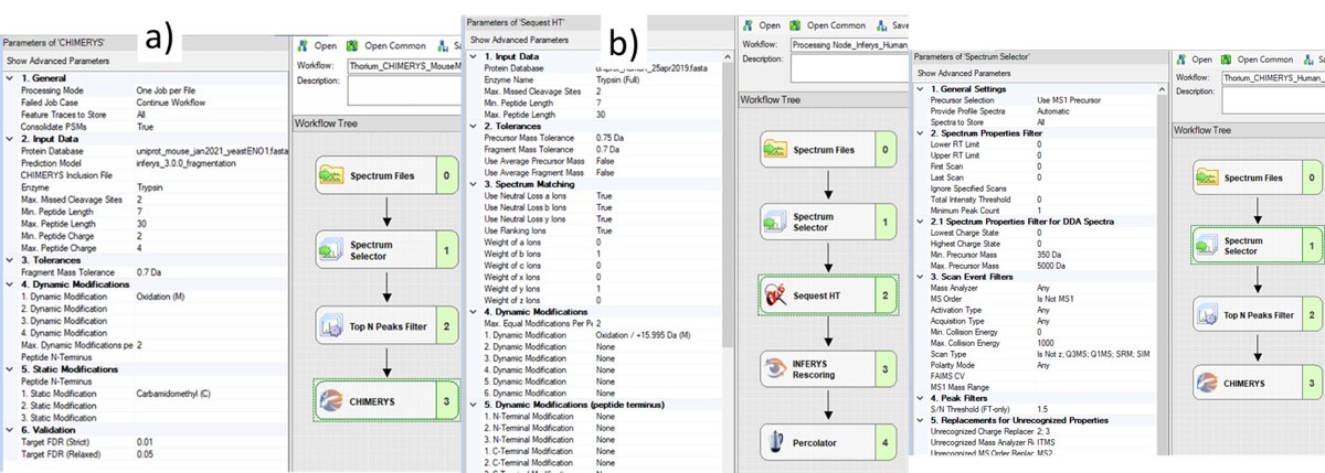
Also, in the spectrum selector node we set the Scan Type to “Is Not Z” (only Full), so that the large isolation width Adaptive RT acquisitions are filtered, which have a Z in the scan header.
A nice, new feature in the Proteome Discoverer 3.1 SP1 is the addition of the Consolidate PSMs option in the Chimerys 1. General section. Setting this parameter to True tells Chimerys to keep on the best PSM per peptide/charge precursor. This consolidation has the effect of speeding up the Consensus workflow significantly, as well as reducing output file size and the amount of time needed for Skyline to import the results.
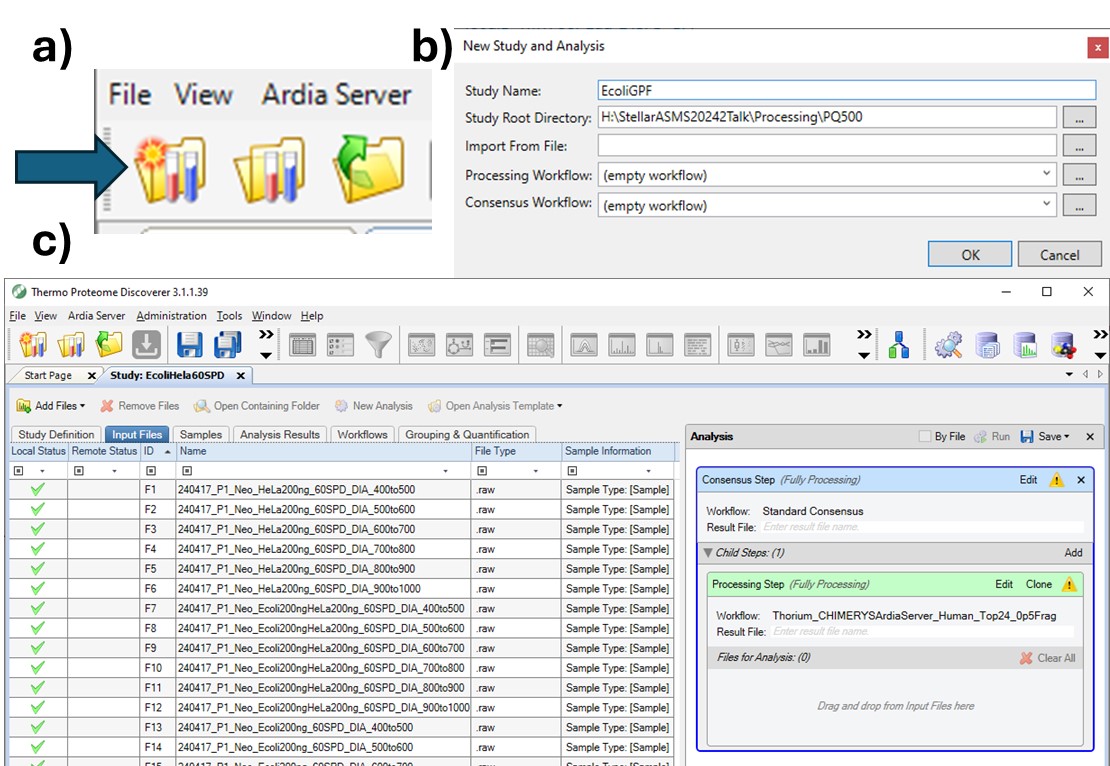
To process the files in Proteome Discoverer, one can first create a study (a), set the study name and directory, and the processing and consensus workflows (b). The workflows can also be set or modified once the study has been created. When the study has been created, one uses Add Files to choose the library raw files, and drags them to the Files for Analysis region, and then presses the Run button to start the analysis (c)
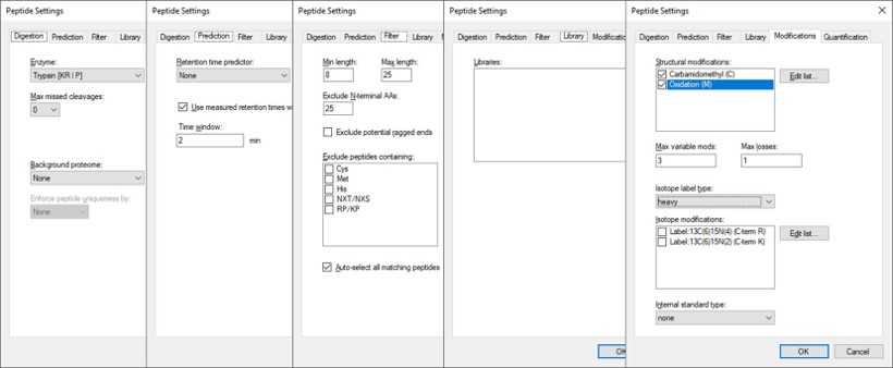
After Proteome Discoverer finishes processing the data, a file is produced with the .pdResult extension, and another one with the .pdResultDetails extension. Both files must be in the same folder for Skyline to import the search results and to start refining a First-Draft targeted method. We will first show you how to import the results manually, and then we will present a simple tool to perform the import with the settings that we recommend for ion trap analysis. To import the PD results manually, create a new Skyline document, and save it as ImportedGPFResults\gpf_results_manual.sky. Open Settings \ Peptide Settings, and set the parameters as in the figure below. The main points are to ensure that no Library is selected, and the Modifications do not specify any isotope modifications. Skyline will check for Structural modifications in the imported search results and ask you about any that are not already specified. Press Okay on the Peptide Settings dialog box.
Open the Settings \ Transition Settings and use settings like below. Set Precursor charges to 2, 3, 4, Ion charges to 1,2, and Ion types to y,b. Don’t specify ‘p’ in Ion types, because PRM Conductor currently takes this as a sign that DDA is being used and loses some functionality. Set Product ion selection from ion 2 to last ion. For Ion match tolerance use 0.5 m/z, with a maximum of 15 product ions, filtered from product ions. Set the Min m/z to 200, and Max m/z to 1500 (whatever was used for acquiring the GPF data), with Method match tolerance of 0.0001. Set MS1 filtering to None, and MS/MS filtering to Acquisition method DIA, Product mass analyzer QIT with Resolution 0.5. For the Isolation scheme, if a suitable scheme is not yet created, select Add. Here we set 0.35 for the Retention time filtering, but a wider window may be more acceptable for longer gradients.
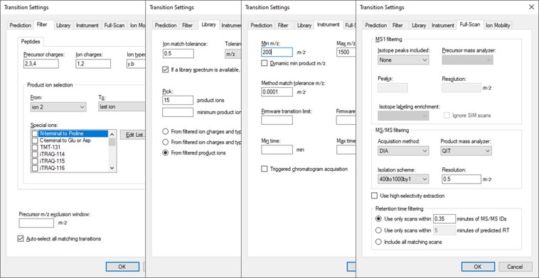
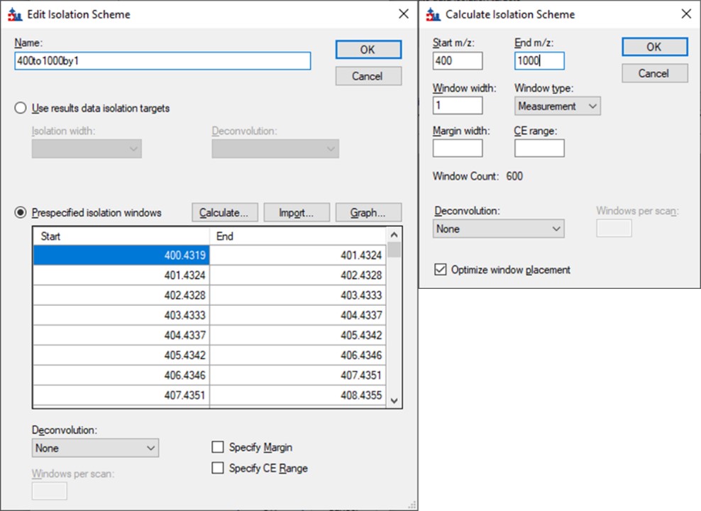
As below, once Add is selected for Isolation Scheme, give it a suitably descriptive name, then press Calculate. Set the Start and End m/z to the limits and isolation width used in the GPF experiment, and click the Optimize window placement button, assuming you used that option in the GPF experiment. Press Ok twice to close the Isolation Scheme Editor, and once more to close the Transition Settings.
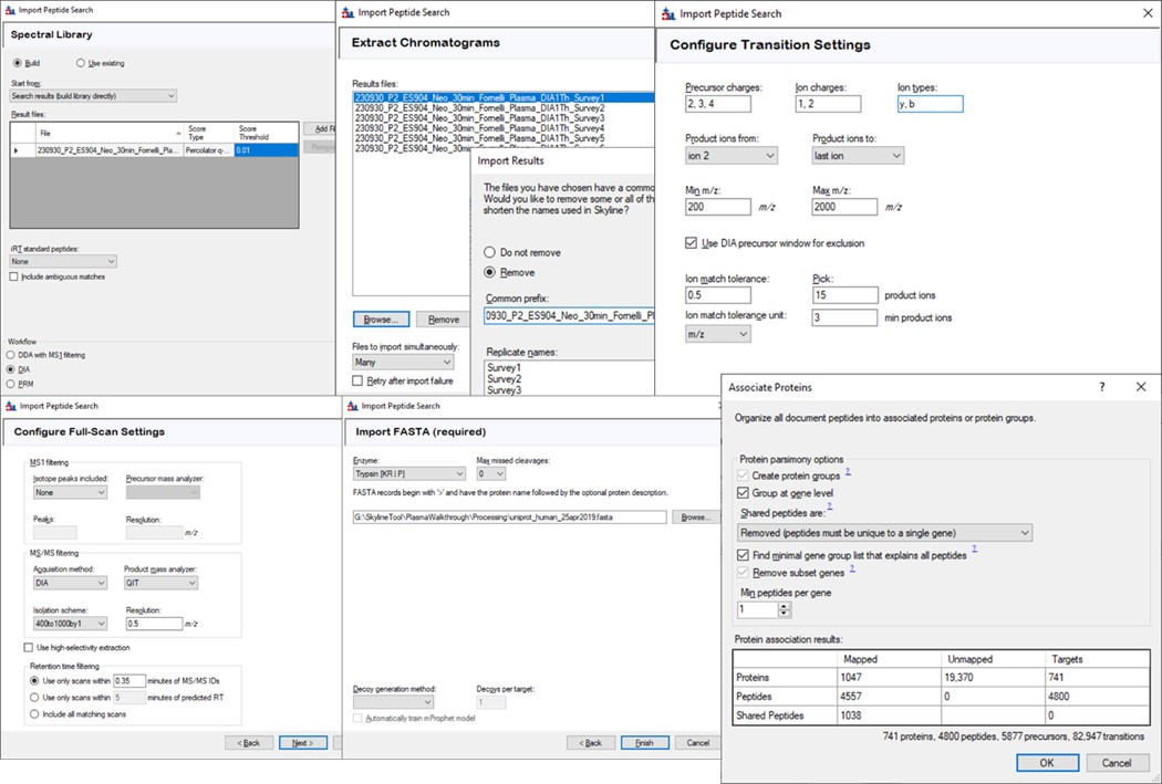
Save your Skyline document at this point, and select File / Import / Peptide Search. Use the Add Files button to navigate to and select the Step 1. DIA GPF/Processing/240417_P1_Neo_Ecoli200ngHeLa200ng_60SPD_DIA.pdResult file.
As in Figure below, select Score Threshold 0.01, Workflow DIA and press Next. Skyline will build a .blib file from the .pdResult, which will take several minutes. If you get an error during this step, ensure that the .pdResultDetails file is also present in the same folder as the .pdResult file, for PD >= 3.1, and ensure that you are using an updated version of Skyline (preferably the Daily version). When this step finishes, Skyline presents a .raw file chooser dialog, select Browse and select the files in Raw / GPF. Press Next, then you can remove or not remove portions of the file names to shorten them, and press Okay. The next Add Modifications tab should be empty if the Peptide Settings / Modifications were already specified, so press Next again. In the Configure Transition Settings, Skyline will have overwritten several of your Transition settings, so remove the ‘p’ from Ion types, and set Ion match tolerance to 0.5, and Max product ions 15, Min 3 and press Next. In the Configure Full Scan Settings, set the MS1 Isotope Peaks to None, and press Next. In the Import FASTA tool, Browse and select the .fasta file in the Processing folder. You can set the Decoy generation to None, especially if you used PSM Consolidation to reduce to a single PSM per peptide, then press Finish. Skyline will start associating peptides to proteins now, displaying a progress bar, and eventually shows an Associate Proteins tool. Here the most strict setting would be to create protein groups and remove any peptides that are not unique to a protein, but alternatively one might choose to Assign to the first gene, for example. Press Okay, and Skyline will import the results from the .raw file, which may take a few minutes. Note that one could have skipped the results importing and pressed cancel at any time after the library was created. The library would be available to browse with View / Spectral Libraries, and the peptides could be added to the document with Add All. Occasionally this process can be used if there were any errors or issues with modifications. Additionally one could use this strategy to load the .raw files as a single multi-injection replicate, the way that the GPF Importer will do, which makes viewing the results much more convenient as we’ll see below. When the results are finished loading, save the gpf_results_manual.sky file.
Click on the second gene labeled greA to expand it. Notice that with the 600to700 file selected, only two peptides are visible. With the scheme we have used, each .raw file was loaded on its own, instead of as part of a whole. To see the difference, use Edit / Manage Results (or Ctrl+R) to open the Manage Results tool, press Remove All and Okay. Now use File / Import / Results. When asked if you want to use decoys say No. In the Import Results tool, select Add one new replicate and use the name GPFMultiReplicate, and press Okay. Choose the six .raw files in the Raw / GPF folder again, and they will be immediately imported if you had finished the importing with the Wizard. The greA gene that is expanded now will have all its peptides completely filled in, like below. Save the gpf_results_manual.sky document.
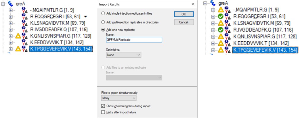
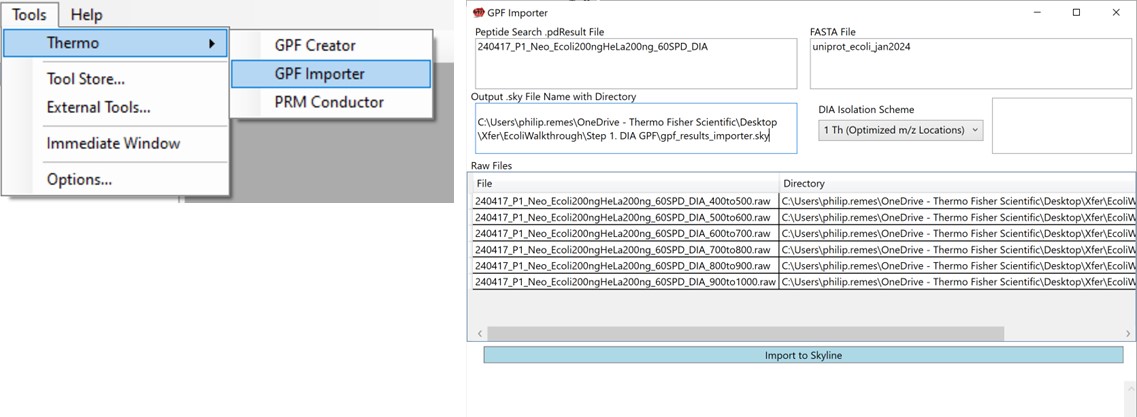
We’ll now look at how the GPF Importer does the same thing as above, but with fewer steps. To use the GPF Importer tool use Tools / Thermo / GPF Importer. Double click the Peptide Search and FASTA file boxes to select the .pdResult file and FASTA file respectively. In the Output file Path, Copy/Paste in the output directory you want, and type an appropriate name for the new Skyline file. Double-click the Raw File pane and select the associated GPF .raw files and press the Import to Skyline button. The log window shows the progress of the import, which takes several minutes. When it finishes, the result will be the same as in the figure below when the multi-injection replicate was imported.
This is the end of the first step. We have Skyline files with peptide search results in them. In the next steps we'll refine the results on our way to making a final assay.
| Attached Files | ||
step1_dia_scheme.jpg step1_dynamic_agc.jpg step1_gpf.jpg step1_gpf_creator.jpg step1_gpf_importer.jpg step1_gpf_template.jpg step1_me_dynamic_agc.jpg step1_pd_analysis.jpg step1_pd_spectrum_selector.jpg step1_sky_pep_settings.jpg step1_sky_trans_settings.jpg step1_tms2_art.jpg step1_tms2_template.jpg step1_pd.jpg step1_manual_import_wizard.jpg step1_multiinject.jpg overview_workflow.jpg