Unscheduled PRM for Neat Heavy PQ500 with Multiple Replicates

In this step, we’ll use Skyline to create a set of unscheduled PRM methods for the 804 PQ500 peptides. At the end of this step, we will have created 10 Unscheduled PRM methods for both 60 and 100 SPD, acquired data for them, loaded the results into Skyline, and assessed the results. We’ll be ready to look at our standards spiked into matrix in the next step.

Alternative DIA GPF Acquisition

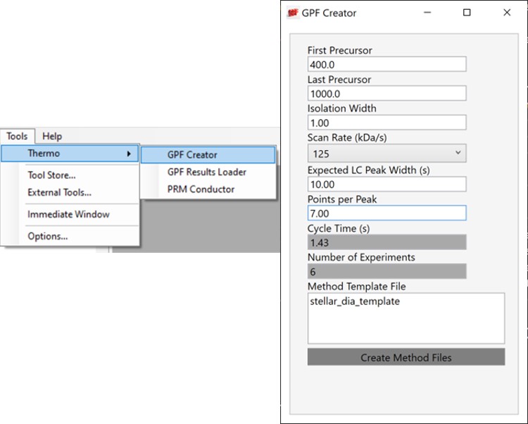
Alternatively, especially as the number of heavy peptides increases, one could opt to use data independent acquisition (DIA) of the neat, heavy standards to find their retention times. One would simply find the smallest and largest m/z of the peptides in question and use the Thermo method editor to create a DIA method. For example, we have had success in some neat standard cases using a single injection with 4 Th isolation width. However multiple gas-phase fractions (GPF) could be acquired with narrower isolation widths, as in the technique we use for identification of unknowns. We included a little helper application in our Thermo suite of external tools called GPF creator that spawns GPF instrument methods. Given a set of parameters, namely a precursor m/z range and a Stellar DIA method template, it will create a cloned set of methods with the appropriate Precursor m/z range filled in. In the case below with Precursor m/z range 400-1000 and 6 experiments, methods would be created for the ranges 400-500, 500-600, all the way to 900-1000. The resulting .raw files could be used in the much the same way that we’ll use the unscheduled PRM data files in the coming steps, only that we would have to configure the Skyline Transition / Full Scan / Acquisition to DIA with the appropriate window scheme (Ex. 400 to 1000 by 1 with Window Optimization On). As it is, we continue on, using the Unscheduled PRM technique.

Creating Unscheduled PRM Methods

The newest Skyline release supports Stellar for exporting isolation lists and whole methods, which is convenient as it saves the step of importing isolation lists for each of the methods. However, for completeness we'll also describe how to use the isolation list dialog with manual import into method files.

Isolation List with Manual Import to Instrument Method Files

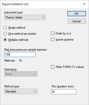
Open the dialog using File / Export / Isolation List. Set Instrument type Thermo Stellar, select Multiple methods, Max precursors per sample injection to 100, Method type Standard. Note that the max value of 100 is approximate. A smaller number could be required for more narrow peaks or shorter gradients. Press Okay.

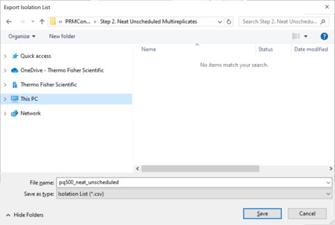
A Save-As dialog will open. Use the name pq500_neat_unscheduled in the folder Step 2. Neat Unscheduled Multireplicates. In a moment, 10 .csv files with the suffix _0001 to _0010 will appear in the folder. An important aspect of the iRT workflow is that Skyline included the PRTC compounds in each of the 10 files. This allows Skyline to calculate the relative positions of the rest of the peaks, which will eventually be added to our iRT library.

Open the Stellar method editor and open the file Step 2. Neat Unscheduled Multireplicates/pq500_60spd_neat_multireplicate.meth. In the tMSn experiment in the bottom right you can find the Mass List table and press the Import button to load the first of the created isolation lists, pq500_neat_unscheduled_0001.csv. Use File / Save-As to save the method as pq500_neat_unscheduled_0001.meth. Do this for each of the other 9 isolation lists, creating a total of 10 methods. At this point you would create an Xcalibur sequence with these 10 methods, injecting an appropriate amount of neat standard (ex 10-100 fmol for a 1 ul/min, 24 min assay), and creating 10 raw files. We have performed this experiment for both 60 and 100 SPD methods, and put the resulting .raw files in the folder Step 2. Neat Unscheduled Multireplicates/Raw.

Skyline Method Export

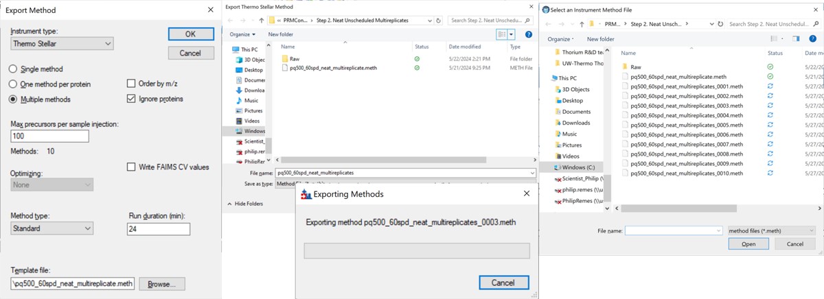
The more convenient way to create the unscheduled replicates is to use the Skyline File/Export/Method functionality. In the Export Method dialog, select Instrument type Thermo Stellar. Select Multiple methods, with Max precursors per sample injection 100. This is a ballpark number that has given enough points per peak for identification purposes for neat standards for a variety of experiment lengths. Click the Browse button and choose the pq500_60spd_neat_multireplicate.meth file in the Step 2. Neat Unscheduled Multireplicates folder. Use a name like pq500_60spd_neat_multireplicates and press Save, and Skyline will present a progress dialog. When it finishes, 10 new methods will be created with suffix _0001 through _0010, as shown below.

Loading Unscheduled PRM Data

Take the .sky file that we have created, Step 1. Setup Skyline Documents/pq500_60spd_neat_multireplicate.sky and use File / Save As to save a copy with the name Step 2. Neat Unscheduled Multireplicates/pq500_60spd_neat_multireplicate_results.sky. If you want to work along with the 100 SPD method as well, you can save another version of the file with the corresponding name.
Use File / Import / Results and select Add one new replicate. Give it the name NeatMultiReplicate. Press Okay, and then select all the raw files in the folder Step 2. Neat Unscheduled Multireplicates\Raw\NeatUnscheduled60SPD and press Open. Skyline will load the results. When they are finished loading, Save the Skyline document. Do the same for the 100 SPD .raw files in their .sky file.

Now we will inspect the results to see if any peaks have been chosen incorrectly. Use File / Save As to save the Skyline document as Step 2. Neat Unscheduled Multireplicates/pq500_60spd_neat_multireplicate_results_refined.sky (and one for the 100 SPD file).
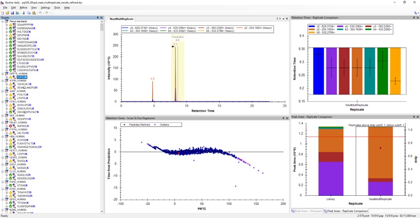
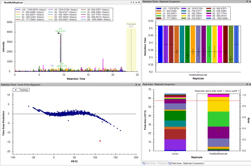
Use View / Retention Times / Regression / Score to Run. Right click the plot and select Plot / Residuals. Right click the plot and make sure that Calculator is set to the calculator that we created, PRTC.
Right click on the plot and select Set Threshold and enter 0.99. If the plot does not update to have some of the blue dots turn pink, then right click the plot and select Plot / Correlation, and then switch back to Plot / Residuals.
Use View / Peak Areas / Replicates Comparison and setup the Skyline document something like in the figure below.

Reviewing the Unscheduled PRM Results

Using Score-to-Run RT Outliers

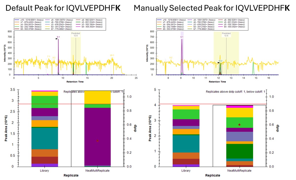
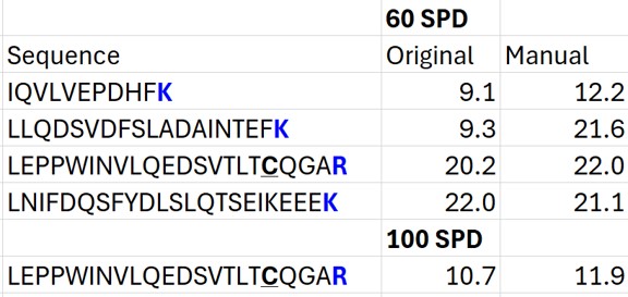
The Residual Score-to-Run plot is very useful for this step to flag any potential missed peaks. Here we want to click on any of the pink "outlier" dots and inspect them. For example the IQVLVEPDHFK was picked at 9.1 minutes, but the peak in the predicted window at 12.6 has a better library dot product match. Also based on the 100 SPD data, we think that the LLQDSVDFSLADAINTEFK is probably the low intensity peak at 21.6 minutes and not the larger peak at 9.3 minutes that is far away from the predicted RT.

Using Dot Products

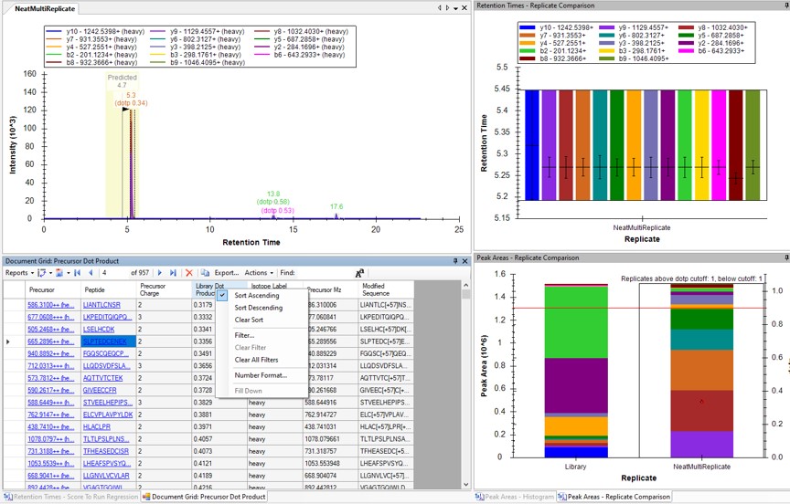
Another way to find picked peak issues like this is to view a Document grid report that has the dot product scores. Use View / Document Grid (or Alt + 3) to bring up the Document grid, and dock it in the same window as the Retention Time Score-to-Run.
- If you ever can't dock a window where you want it, dock the window in some place that Skyline lets you, and then you will be able to dock it where you originally wanted.
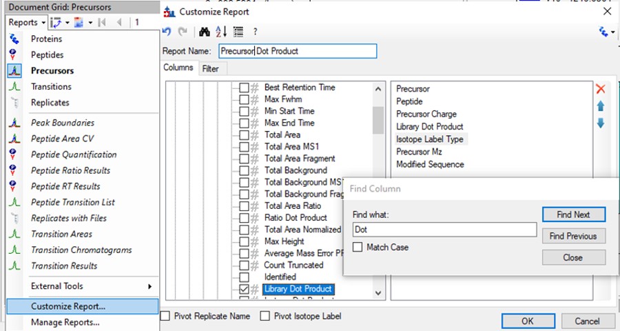
Click the Precursor Report, then Customize Report to bring up a dialog menu. Erase columns from the right hand side and then click the binoculars and type 'Dot', and press Find Next until you find Library Dot Product. Select this column to add it to the right hand side, and then press okay.

Now right click on the Library Dot Product column and select Sort Ascending. You can click through on the worse dot product scores to inspect them. Even the ones with poor dot product scores are actually pretty ambiguously belonging to a single precursor at the correct retention time.

Using Peak Picking Models

A final way that can be useful for inspecting this kind of result is to compare the results from the two Skyline peak picking models available at this time. Although in the present case there is not much use for this technique, we'll demonstrate it now.

Select Refine / Reintegrate. In the Peak scoring model dropdown box, select Add. In the dialog that shows up, keep mProphet as the model, and select Training / Use second best peaks. Using decoys is the method used when you have DIA data and have added Decoy peptides to the document. For targeted methods, the second best peak for the peptide serves as the null distribution for training the peak model. Click Train Model. In the feature scores there are several scores that are not available because there are no light peptides in the document. Scroll down the see the enabled features. Several features are red because they decreased the classification accuracy. Unselect those features and press Train Model again, and click Okay to exit the Edit Peak Scoring Model dialog.

In the Reintegrate dialog, Add another peak scoring model. This time select the Default model and press Train Model. Then press Okay, and press Okay again in the Reintegrate dialog. This should give us the original peaks selected when the data were imported.

Go to Refine / Compare Peak Scoring. Use the Add button to add the two peak models that we just made. Go to the Score Comparison tab, select the Default model for the Compare dropdown and the mProphet model for the "with" dropdown. Click the Show conficts only button. Of the 8 conflictin peaks, the greatest ambiguity is probably the first one, LLGNVLVCVLAR. Here there is a very nice peptide peak at 20.9 minutes, but the one at 20.5 although it is further from the predicted RT, has a better dot product. We selected the 20.9 peak, but potentially this is misassigned. We made the same assignment in the 100 SPD method.

Summary of Changes made to Default Skyline Peak Picking

The figure below summarizes the manual changes we made to the Skyline default peak picking. Note that at the time that we first did the study, Skyline could connect to the Prosit server for library generation. By the time this tutorial was written, Skyline was using something called Koina to do the in silico predictions. While the Prosit models are in theory supported, there was an issue with using them. Therefore there could be some small differences. Note that the most conservative approach would be to search the unscheduled PRM data against a PQ500 .fasta file with static R and C heavy modifications, and only select those peptides that passed some threshold FDR value.

Saving a New, Empirical iRT Calculator

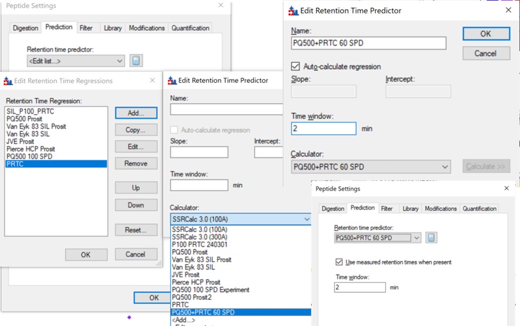
Now we will update the iRT library so that future experiments can benefit from this curated peak picking. Use Settings / Peptide Settings / Prediction, and click the calculator button to Edit Current. In the dialog that opens, click Add in the bottom right corner and add results.., and an Add iRT Peptides dialog announces that 804 peptide iRT values will be replaced. Click Okay. Click Yes when asked if the iRT Standard values should be recalibrated. Now in the iRT database line, use the name pq500_60spd.irtdb, and give it a new name, PQ500+PRTC 60 SPD, press Okay to exit.

We've created a new iRT calculator, but have to set it as the active one. Click the calculator icon and Edit List. Press the Add button and then click the dropdown menu, and the new calculator will be there, select that one. Set the Time window to 2 minutes, then press Okay. Select the PQ500+PRTC 60 SPD calculator in the Peptide Settings / Prediction dialog and press Okay to exit to main Skyline window.

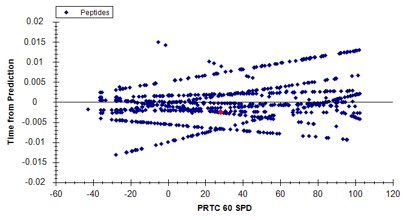
In the score-to-run plot, right click, select Calculator, and choose the PQ500+PRTC 60 SPD. The plot will update to show an interesting pattern where the errors are all very close to zero. We have now created a new calculator that will make it easier for Skyline to pick peaks next time. We did the exact same set of iRT steps for the 100 SPD Skyline file, because using the new 60 SPD calculator for the 100 SPD does not work perfectly. In the 100 SPD we think that probably the LEPPWINVLQEDSVTLTCQGAR is the peak at 11.9 minutes and not the one at 10.7 minutes.

Filtering Transitions with PRM Conductor

This was a neat sample, but we can filter out the transitions that we don't need at this point, with the understanding that when we spike into plasma we may have to refine the transitions even further.

Select Tools / Thermo / PRM Conductor. The tool opens up. We used the settings in the figure below, where importantly you set Min Good Trans to 5, press Enter, and also select the Keep All Precs box. Press the Send to Skyline button on the bottom left. Save the Skyline document and close the PRM Conductor.

The number of transitions displayed in the bottom right hand of Skyline will have updated. With the settings we used, the number of transitions dropped from 11,088 to 7,564.

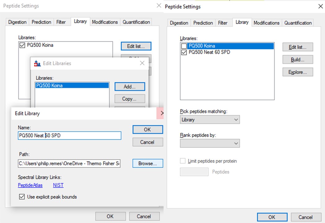
Use File / Export / Spectral Library and save as Step 2. Neat Unscheduled Multireplicates/PQ500_Neat_60SPD_Refined. Use Settings / Peptide Settings / Library and select Edit List, then Add, and Browse for the file you just saved. Give the library the name PQ500 Neat 60 SPD. Press Okay, and in the Library tab, deselect the PQ500 Koina library and select the new library. Press Okay and save the Skyline document. Make a spectral library in the same way for the 100 SPD document. Close the PRM Conductor instances. We've reached the end of the second step, and are ready to acquire data in plasma.