Table of Contents |
guest 2025-07-02 |
GPF Creator
GPF Importer
PRM Conductor
Expert Review
Sequence Import Configure
Thermo External Tools Overview
Introduction
As of mid-2025, the Thermo set of External tools downloaded under the name PRM Conductor includes 5 different tools
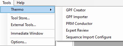
- GPF Creator
- an small application that automates the creation of multiple instrument method DIA files to span a precursor range for a gas-phase-fractionation experiment
- GPF Importer
- a small application that automates the import of GPF or any peptide search data from Proteome Discoverer. This program imports the data with defaults that are appropriate for the Stellar MS, but the same result can be achieved through the Skyline File / Import / Peptide Search wizard.
- PRM Conductor
- an application that aids in the creation of targeted MS methods. This program filters "bad" transitions, and selects "good" peptides via a set of criteria, and helps the user to create one or more instrument methods that will be acquired with at least a required number of points per peak.
- Expert Review
- an application that helps achieve consistent peak integration boundaries, through the use of replicate-level and experiment level correlations to reference data of various types.
- Sequence Import Configure
- a tiny application that saves a file on the instrument computer, which allows to automatically import .raw files into a Skyline file after the .raw file acquisition is finished
GPF Creator
GPF Creator Quick Reference
GPF Creator is small application that automates the creation of multiple instrument method DIA files to span a precursor range for a gas-phase-fractionation experiment.
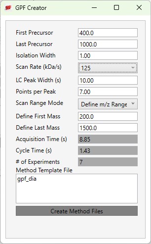
- First Precursor
- The lower bounds precursor m/z
- Last Precursor
- The upper bounds precursor m/z
- Isolation Width
- The quadrupole mass filter isolation width. The precursor range is split up into a series of acquisitions having this stride.
- Scan Rate (kDa/s)
- The ion trap mass analysis rate. This value determines how fast the acquisitions are acquired, and affects the number of experiments needed to span the precursor range.
- LC Peak Width (s)
- The expected LC peak width at the base. The cycle time is this value divided by the desired points per peak.
- Points per Peak
- The minimum acquired points per LC Peak width. The cycle time is the LC peak width divided by this value.
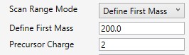
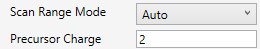
- Scan Range Mode
- Define m/z Range
- Define an explicit first and last mass for the acquired spectra. The acquisition rate is inversely proportional to the size of the m/z range.
- Define m/z Range
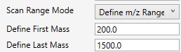
- Define First Mass
- Define a constant first mass for all acquisitions. The last mass is determined based on the charge state, such that last_mass = precursor_mz * charge + 10
- Auto
- The first and last mass are determined automatically. The last mass is determined as in the Define First Mass mode. The first mass is determined as the lowest mass that still retains most of the ions at the last mass, based on experimental evaluations.
- Acquisition Time(s)
- The total estimated amount of time to acquire data for all the acquisitions from the First Precursor to the Last Precursor, with the given settings. The # of Experiments is this value divided by the Cycle Time, rounded up to the next integer.
- Cycle Time (s)
- The desired cycle time, based on the LC Peak Width / Points per Peak
- Number of Experiments
- The total number of experiments required to span the Precursor range with the current settings. This is the number of instrument methods that will be created when Create Method Files is clicked.
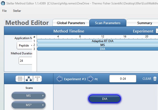
- Method Template File
- Double click this text box to open a file chooser for instrument .meth files. The file should have at least one DIA experiment, not counting Adaptive RT experiments (ART). The first non-ART experiment will be modified in the newly created files. The method should have all the LC details desired, and have the appropriate Method Duration and Experiment Durations.
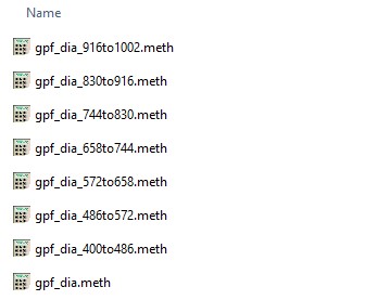
- Create Method Files
- Click this button to create the instrument methods. Each method will have the name of the template method, with the precursor mass range appended to the end. For example for the gpf_dia.meth template method, files with names like gpf_dia_572to658.meth are created.
GPF Importer
GPF Importer Quick Reference
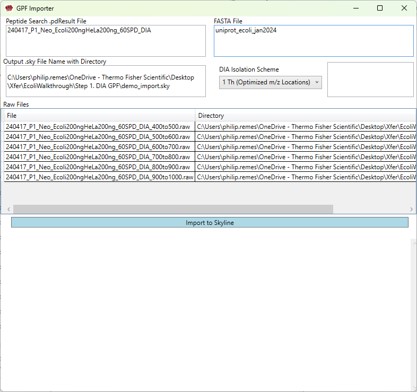
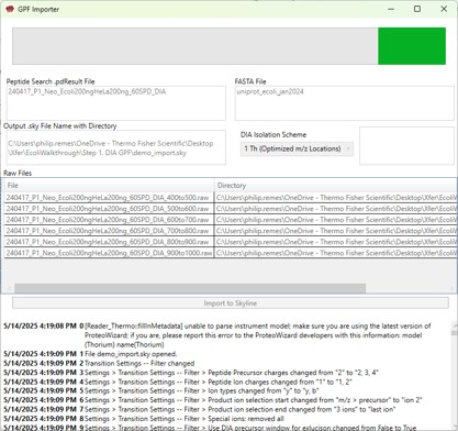
GPF Importer is a small application that automates the import of GPF or any peptide search data from Proteome Discoverer. This program imports the data with defaults that are appropriate for the Stellar MS, but the same result can be achieved through the Skyline File / Import / Peptide Search wizard.
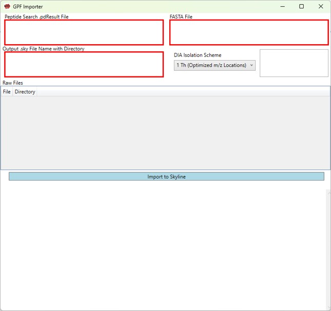
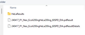
- Peptide Search .pdResult File
- Double click to open a file chooser for a .pdResult file. Since PD v3.1, a corresponding file with the .pdResultDetails extension must be present in the same folder.
-
Fasta File
- Double click to open a file chooser for a .fasta file.
-
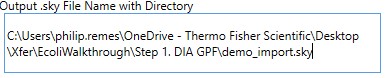
Output .sky File Name with Directory
- Enter the full path to where you want the output .sky file to be. The folder must exist, and the extension of the file must be .sky for the red outline around the box to go away. Usually one can copy the path to a folder and paste here, and then type the desired .sky file.
- Enter the full path to where you want the output .sky file to be. The folder must exist, and the extension of the file must be .sky for the red outline around the box to go away. Usually one can copy the path to a folder and paste here, and then type the desired .sky file.
-
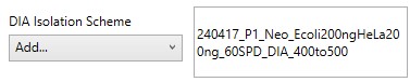
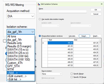
DIA Isolation Scheme
- Select the isolation width used for your experiment. The chooser assumed that you used the Window Placement Optimization option in the Method Editor.
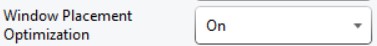
- Select the isolation width used for your experiment. The chooser assumed that you used the Window Placement Optimization option in the Method Editor.
If for some reason, you didn't use Window Placement Optimization in the DIA method, it's possible to select a .raw file that has the DIA isolation scheme that you want to do. This is equivalent to using Skyline to Add an isolation scheme, and selecting Import.
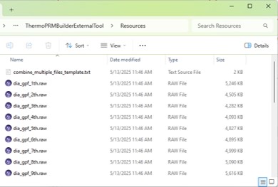
The GPF creator does this for the pre-defined schemes, by creating a short 1 minute instrument method with a scheme, and acquiring the .raw file through Tune. You can find the template raw files if you can find the installed Skyline Tools directory by inspecting the Skyline Immediate Window when you launch a tool.
-
Raw Files
- Double click this box to select one or more .raw files that will be imported to the created .sky file after the spectral library is created from the .pdResult files.
- Double click this box to select one or more .raw files that will be imported to the created .sky file after the spectral library is created from the .pdResult files.
-
Import to Skyline
- Click this button to start the import. As the import happens, the Skyline API logging text will print to the lower text box.
- Click this button to start the import. As the import happens, the Skyline API logging text will print to the lower text box.
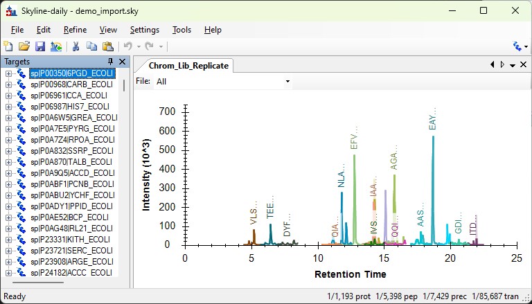
Once the import is finished (it can take minutes), the output skyline file will open, with all the data imported. You would be ready to create an assay with PRM Conductor next.
PRM Conductor
PRM Conductor Quick Reference
PRM Conductor is an application that aids in the creation of targeted MS methods. This program filters "bad" transitions, and selects "good" peptides via a set of criteria, and helps the user to create one or more instrument methods that will be acquired with at least a required number of points per peak.
Launching PRM Conductor from the Thermo tools menu will open the application. If there was data in the Skyline document, a report will be exported from Skyline and imported to PRM Conductor. The view will look similar to below.
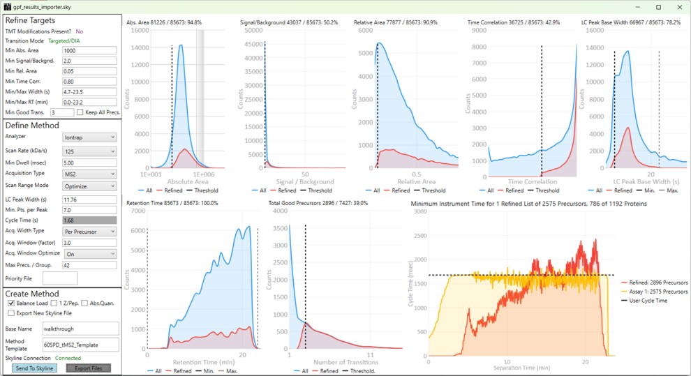
The user parameters are split into 3 sections; Refine Targets, Define Method, and Create Method
Refine Targets
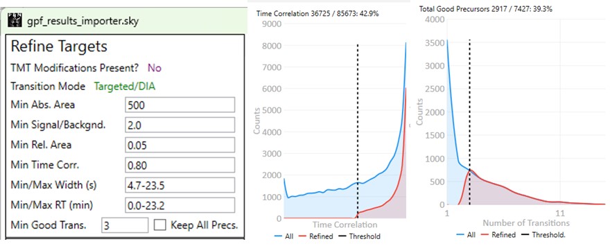
These parameters configure a series of simple filters for the transitions, and allows to filter precursors by the number of good transitions that they have.
- TMT Modifications Present?
- This value is No if there are no TMT modifications. If TMT modifications are present, then the exported methods can account for this, for example by choosing MS3 precursors that have TMT tags.
- Transition Mode
- This value is Precursor/DDA if ALL the analytes have precursor transitions. The 1.0 PRM Conductor version would set this mode if ANY precursor transition was present, which was confusing. This DDA mode means that MS2 data may only be acquired once per LC peak, and so some metrics like Time Correlation are not valid. This mode is common for Small Molecule analysis when data are imported from Compound Discoverer. PRM Conductor is still useful in this case, to create instrument methods, but it may be advisable to select Keep All Precs. option, and apply filtering on a later targeted data set.
- This value is usally Targeted/DIA, enabling the full filtering functionality of the Time Correlation filter.
- Min. Abs. Area
- Filters transitions by requiring that they have a minimum absolute area value. This value may have to change for data acquired on different instruments. For example, the intensity scaling on Orbitrap instruments is arbitrarily scaled to a value that is ~10x the value for Ion trap and Astral data.
- Min. Signal / Backgnd.
- Filters transitions by requiring that they have a minimum signal to background ratio. Signal is the Skyline peak area, and Background is the Skyline background value. This value should be used sparingly, because the current background metric that we use is not as good as it could be.
- Min. Rel. Area
- Filters transitions by requiring that they have a minimum relative area to the largest transition for its precursor.
- Min. Time Corr.
- Filters transitions by requiring that they have a minimum correlation to the median transition. This value is called Shape Correlation by Skyline,and was defined by Searle et. al., and later in some detail by Heil et. al.
- Min./Max. Width (s)
- Filters transitions by requiring that their base LC width be within the given bounds. The bounds is computed from the Skyline FWHM and converted to a base peak width by assuming a Gaussian shape and multiplying by 2.54. See the supplement of Remes et. al. for a derivation.
- Min./Max. RT (min)
- Filters precursors by requiring that their retention time be within the given bounds.
- Min. Good Transitions
- Filters precursors by requiring at least this many transitions that satisfy the above filters.
- Keep All Precs.
- This option ensures that no precursors are filtered, and the top Min. Good Transitions are kept. If there are not enough good transitions, "bad" transitions are selected according to Area x Time Corr. This option is useful when the user wants to keep all the precursors and just clean up the transitions, or is using DDA mode.
Define Method
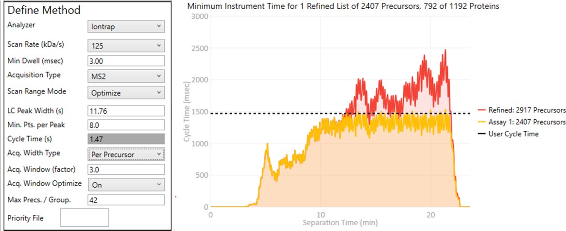
These parameters control how many targets can be included in the assay. When parameters in this section are changed, and the 'enter' key is pressed, the graph on the right will update, showing how many precursors can be included in the assay, while respecting Cycle Time defined by the LC Peak Width and the Min. Pts. per Peak.
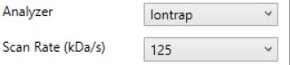
Analyzer
- Ion Trap
- Scan Rate (kDa/s)
- Sets the analysis scan rate. This value affects the acquisition rate, and therefore the assay target capacity.
- Scan Rate (kDa/s)
-
Astral
- Currently the Astral has no analyzer-specific parameters
- Currently the Astral has no analyzer-specific parameters
-
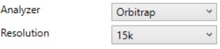
Orbitrap
- Resolution (k)
- Sets the analysis resolution. This value affects the acquisition rate, and therefore the assay target capacity.
- Sets the analysis resolution. This value affects the acquisition rate, and therefore the assay target capacity.
- Resolution (k)
-
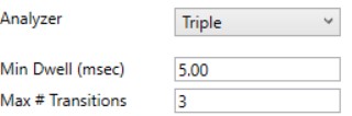
Triple
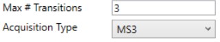
- Max #Transitions
- Only up to this number of transitions will be selected, since this value linearly decreases the assay target capacity.
- Only up to this number of transitions will be selected, since this value linearly decreases the assay target capacity.
- Max #Transitions
-
Min Dwell (msec)
- Also called injection time on many instruments, this value sets the smallest amount of precursor accumulation time per target. Typically we set this value small enough so that it does not affect the assay capacity, and rely on the dynamic AGC algorithm to boost the injection time according to the available time in the cycle. See Remes et. al. for a description of the dynamic AGC process.
- In some cases, the experimenter may know that to achieve high quality data, a minimum dwell time is needed, and will adjust this value accordingly.
Acquisition Type
- MS2
- The standard analysis type, where each acquisition contains data for a single precursor that is mass selected and fragmented.
- MS3
- Currently only available when Ion Trap analyzer is selected, in this mode, each acquisition contains data for a single precursor that is mass selected, fragmented, and one or more fragments are further mass selected and fragmented.
- The Max # Transitions parameter becomes available in this mode, limiting the number of MS3 precursors that will be simultaneous mass analyzed in the second MS stage. For purposes of the acquisition rate estimations, this mode currently assumes that resonance CID with 4 msec activation time is used for the first activation, and HCD is used for the second activation. In reality if the user selects a method template the uses resonance CID for the second activation, then the activation for each MS3 precursor is performed serially, taking at least #transitions x activation_time to be performed.
-
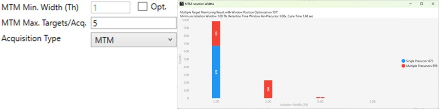
MTM
- Multiple target monitoring is a type of method that can be generated from 1 Th isolation window GPF DIA data. It analyzes the GPF data to determine when it is safe to expand the number of targets, or the isolation width, to encompass multiple targets. MTM can be used to expand the number of targets in an assay compared to normal PRM, or alternatively for the same number of targets, MTM can enable the use faster gradients and higher throughput, or higher injection times and better sensitivity.
- When the Opt. check box is unchecked, then the isolation widths are multiples of the GPF isolation width, which is shown in a disabled text box (1 here). A pop-up window shows the distribution of isolation widths, and how many of them are for single or multiple targets.
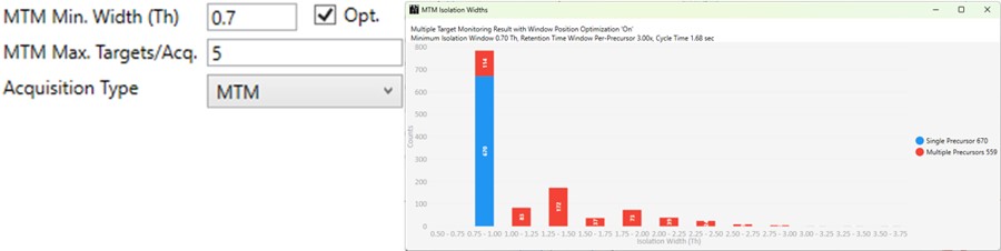
- When the Opt. check box is checked, then the isolation widths are customized for each acquisition, such that the window size is (largest_mz - smallest_mz) + MTM Min. Width (Th).
-
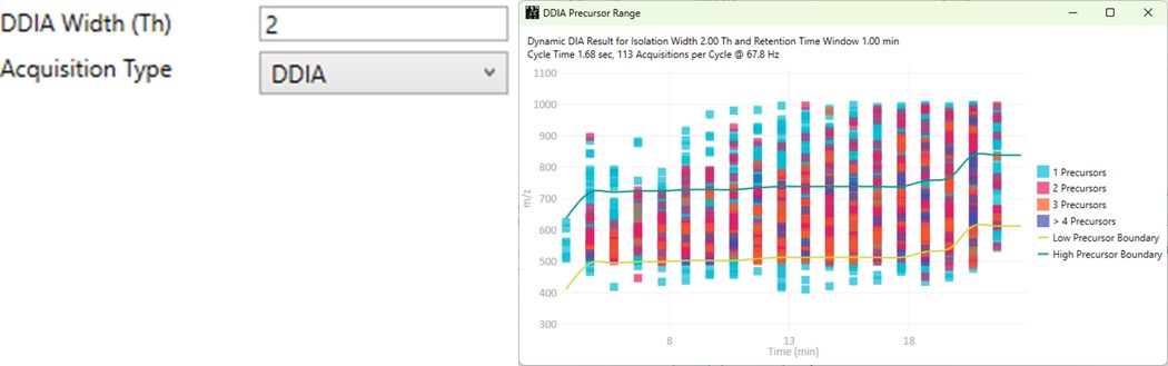
DDIA
- Dynamic DIA is a type of DIA method in which the precursor range shifts as a function of the experiment time. This method can be used to acquire data with a narrower isolation window than would be possible if data for the entire precursor range had to acquired on each cycle.
- The DDIA Width(Th) sets the isolation width that will be used. Narrower widths will acquire higher quality data, for fewer precursors.
- A pop-up plot appears that shows the density of precursors in the Skyline document, along with lines that trace the proposed precursor range as a function of experiment time.
Scan Range Mode
-
Define m/z Range
- Define an explicit first and last mass for the acquired spectra. The acquisition rate is inversely proportional to the size of the m/z range.
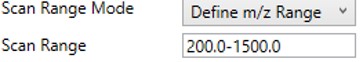
- Define an explicit first and last mass for the acquired spectra. The acquisition rate is inversely proportional to the size of the m/z range.
-
Define First Mass
- Define a constant first mass for all acquisitions. The last mass is determined based on the charge state, such that last_mass = precursor_mz * charge + 10
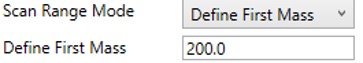
- Define a constant first mass for all acquisitions. The last mass is determined based on the charge state, such that last_mass = precursor_mz * charge + 10
-
Auto
- The first and last mass are determined automatically. The last mass is determined as in the Define First Mass mode. The first mass is determined as the lowest mass that still retains most of the ions at the last mass, based on experimental evaluations.
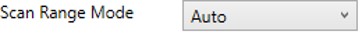
- The first and last mass are determined automatically. The last mass is determined as in the Define First Mass mode. The first mass is determined as the lowest mass that still retains most of the ions at the last mass, based on experimental evaluations.
-
Optimize
- The first and last mass are set based on the set of "good" transitions for a precursor plus a small buffer. This mode enables the fastest acquisition rates possible for the Ion trap analysis, where the mass analysis time is directly proportional to the scan range.
- The first and last mass are set based on the set of "good" transitions for a precursor plus a small buffer. This mode enables the fastest acquisition rates possible for the Ion trap analysis, where the mass analysis time is directly proportional to the scan range.
Other Define Method Parameters
-
LC Peak Width (s)
- The expected LC peak width at the base. This value is pre-populated from the input data, but can be updated as desired. The instrument maximum cycle time is this value divided by the desired points per peak.
-
Points per Peak
- The minimum desired acquisition points per LC Peak width. The cycle time is the LC peak width divided by this value.
-
Cycle Time (s)
- The desired cycle time, based on the LC Peak Width / Points per Peak
-
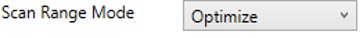
Acquisition Width Type
Defines the method used to set the acquisition window width around each target in the method.- Global
- All targets get the same, global acquisition window size, Acq. Window (min).

- All targets get the same, global acquisition window size, Acq. Window (min).
- Per precursor
Each target gets an acquisition window width defined as its individual base peak width, times the Acq. Window (factor) value.
- Global
-
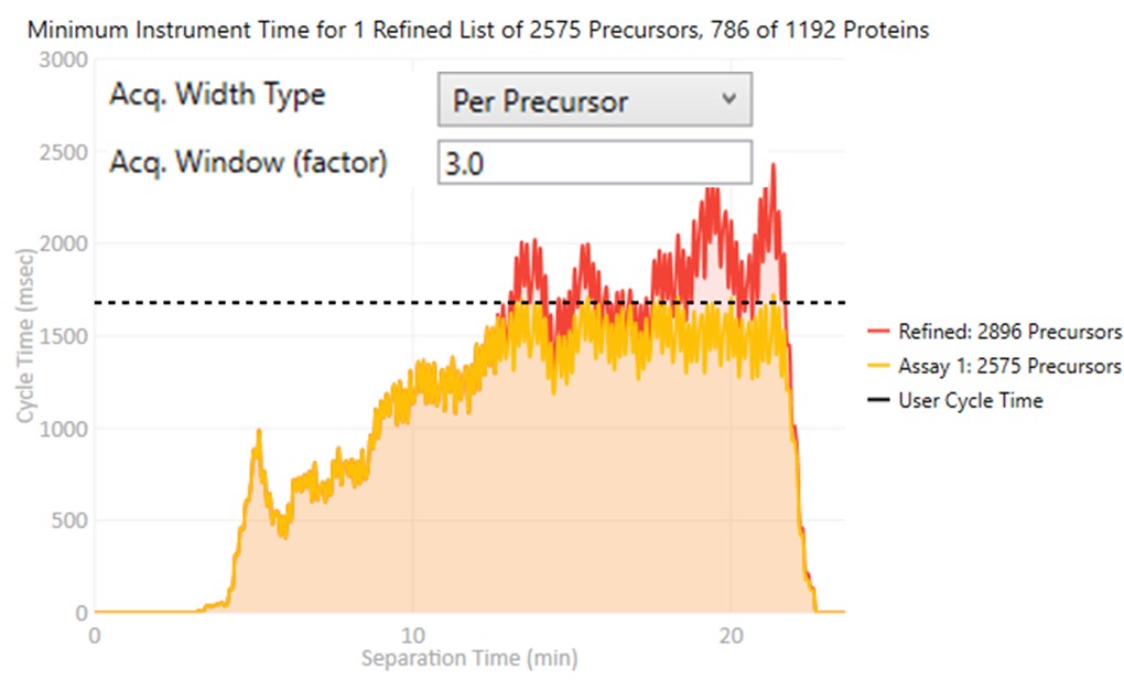
Acq. Window Optimize
- When set to Off, the acquisition windows will be exactly the ones determined based on the current Acquisition Width Type. Note how the Assay 1 density in yellow is the same as the Refined density in red in the time region from 0 to ~10 minutes.
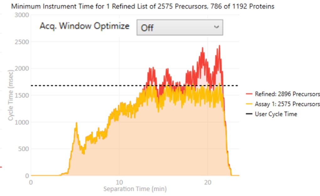
- When set to On, then the acquisition windows widths are expanded by up to some factor (5x currently), while ensuring that the acquisitions don't exceed the desired cycle time. Note how the Assay 1 density matches the cycle time for much of the region between 0 and 10 minutes now. The reason for this mode is that early eluting molecules can have variable retention times, and Adaptive RT may have little information to be able to adjust the targeted schedule at these early times. Making the widths larger in a dynamic way is a nice way to make the assay acquisition more robust. In the future we could add a UI parameter that specifies the maximum expansion factor.
- When set to Off, the acquisition windows will be exactly the ones determined based on the current Acquisition Width Type. Note how the Assay 1 density in yellow is the same as the Refined density in red in the time region from 0 to ~10 minutes.
-
Max Precs. / Group
- Sets the maximum number of peptides per protein in Skyline's Peptide mode, or molecules per molecule group in Skyline's Molecule mode. This parameter can be used to increase assay quality by removing targets from the assay that may not add additional information. The included targets are selected by their quality, defined as their Area x Time Correlation.
-
Priority File
- Double click to select a file with a .prot extension that you've made. Just create a text file, and save it with the .prot extension. On each line, you can enter a protein name, or molecule list name. Skyline puts either the protein name or molecule list name in the Report column called "Molecule List". Any precursors that belong to the protein or molecule list will be accepted into the assay, even if they don't pass all the filters.
- Using a Priority file is a good way to incorporate iRT compounds into an assay, when doing an initial search for heavy-labeled standards.
- If the Balance Load check box is not checked, then each of the multiple assays that may be generated will contain the prioritized targets.
- New for v1.1, you can also enter peptide sequences or molecule names. These are the values found in the Skyline report columns called, "Modified Sequence Monoisotopic Masses", or "Molecule", in the Skyline Protein or Molecule modes, respectively.
- For example, the file could have 2 peptide sequences and a protein name.
LPALFC[+57.021464]FPQILQHR
ESYGYNGDYFLVYPIK
SPEA_ECOLI
Create Method
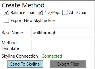
These parameters control aspects of how the method will be created.
-
Balance Load
- When checked, a single assay will be created that respects the currently defined Cycle Time. The number of Refined precursors added will depend on the particular choice of Define Method parameters. Precursors are added to the assay iteratively from each protein or molecule group in turn, where the precursors from each group are added in order from highest to lowest quality. Quality is currently defined as area x time correlation. A balanced load refers to how the precursor time density becomes uniform at the limit of many potential precursors, instead of peaked in the middle of the run.
- When not checked, multiple assays will be created that analyze all Refined precursors. Each assay will be of the traditional, non-balanced type. If a Priority File is specified, prioritized precursors will be added to all of the assays.
-
1 Z/Pep.
- When checked, only a single precursor from each peptide (or molecule, in Skyline's Molecule mode) will be accepted into the assay. The selected precursor will have the highest quality, defined as area x time correlation.
- When not checked, multiple precursors having different charge states could be in the assay, if they all passed the various filters.
-
Abs. Quan.
- When checked, a light-version of each heavy-labeled peptide will be added to the assay. This is a nice way to create a light+heavy assay from an initial heavy-only assay. The instrument time plot will update to have 2x the number of targets, allowing to visualize whether enough points per peak will be acquired.
-
Export Skyline File
- When checked, a new Skyline file having the precursors with their corresponding filtered transitions will be created when the Export Files button is pressed. Because creating the new Skyline file takes some 10's of seconds, it can be annoying, and it was made into an option. The good part about using this option is that the new Skyline file will have its Transition Settings set to PRM with Stellar-specific parameters.
- When not checked, no new Skyline file will be created when the Export Files button is pressed. Often we use this mode, and rely on using the Sync to Skyline button to update the current Skyline document, and later save a new Skyline document manually.
-
Combine DIA Windows for Reference
- This is a special option that only appears if the input data are DIA with isolation width less than 15 Th, and no large window Adaptive RT information is available.
- When checked, and if the .meth has specified Adaptive RT for Dynamic Time Scheduling, then the exported method will have an rtbin file that is made by combining acquisitions in silico. The DIA alignment acquisitions will have an isolation width of near 50 Th, and will adjust the target schedule accordingly.
- This is a nice option when creating Stellar MS targeted assays from Astral DIA data, which are likely acquired with small isolation widths, such as 2, 3, or 4 Th.

-
Base Name
- Output files will have this value in them. For example, the .meth, .sky, and .csv files associated with a method will all have use this name.
-
Method Template
- Double click this text box to open a file chooser for a .meth file that will serve as a template for exported assay files. The template file should have a tMSn method in it, and the appropriate LC parameters, and Method and Experiment durations. Other parameters like activation type should also be specified. If Adaptive RT is specified in the Dynamic Time Scheduling, then an rtbin file will be created during export and saved in the .meth file. This is the preferred way to add Adaptive RT functionality to a method.
- You can make methods on your non-instrument computer if you have downloaded the Workstation version of the instrument software. This software is available at the Thermo Flexnet site.
- In this case, you can use the standalone method editor found at C:\Program Files\Thermo Scientific\Instruments\TNG\Stellar\1.1\System\Programs\TNGMethodEditor.exe.
- The standalone method editor only has access to MS information, not the LC driver information, but you can copy a .meth file from an instrument that has the LC information in it, and then resave and modify it on your laptop.
-
Sync to Skyline
- Pressing this button updates the current Skyline file by filtering the transitions, precursors, and proteins that are not in the final assay.
-
Export Files
- Pressing this button will export precursor lists, transitions lists, .meth files if specified in the Method Template field, and a .sky file if Export to Skyline is checked.
Expert Review
Expert Review Quick Reference
Expert Review is an application that helps achieve consistent peak integration boundaries, through the use of replicate-level and experiment level correlations to reference data of various types.
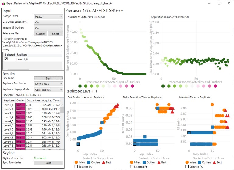
Input
These parameters change how the calculations will be performed. They take affect once the Results:Start button is pushed.
- Isotope Label
Determines whether a specific isotopically-labeled version of the precursor is used for setting the boundaries. Skyline's Isotope Label Type report column is used as input data.- Not Specified
- The isotope label type is not considered. Use this mode for label-free experiments. If this mode is used for data with light and heavy labels, the boundaries that are actually used could come from either molecule (not recommended).
- Heavy
- The integration boundaries from the heavy labeled precursors will be sent to Skyline.
- Light
- The integration boundaries from the endogenous, or light, precursors will be sent to Skyline.
- Not Specified
- Use Other Label's Info
- This parameter is only visible if the Isotope Label parameter is set to Light or Heavy.
- On
- Experiment-level replicate analysis will use information from the other label when attempting to place consistent integration boundaries. Ex. information from the light precursor is used to help determine the heavy precursor boundaries.
- We recommend to use "On", but include this option in case the light data are not consistent between replicates and are hampering the boundary location accuracy.
- Off
- Experiment-level replicate analysis will not use information from the other labeled precursor.
- Impute RT Outliers
- On
- Uses a local regression analysis of retention time and raw file acquisition time to attempt to identify and correct retention time outliers.
- This algorithm is applied after the cross-corrleation based experiment-level replicate analysis.
- This algorithm uses information from the retention times and acquisition times "best" replicates. If these best replicates are all acquired at the start of an experiment, and there is later significant RT drift, the algorithm is not very accurate.
- This algorithm can be useful if there are retention time drifts that vary smoothly with acquisition time. Only use this mode if there are no abrupt shifts in retention time between replicates. Such shifts will cause this algorithm issues.
- Off
- No local regression analysis of retention time and raw file acquisition time is used. The cross correlation-based experiment-level analysis is still used, however.
- On
- Reference File
Expert Review relies on information from a reference replicate or replicates to perform integration boundary determination. The reference can be currently be selected in two ways.- Current
- Select this button to update the Replicates grid with information from the current Skyline file.
- Select
- This button will open a file chooser, whereupon the user can choose another Skyline file to use as a reference. This can allow for faster processing, since the reference data can be smaller and load faster. The only gotcha is that if your reference file transitions for some reason don't overlap with the experiment transitions, or there were precursors in the experiment file that aren't in the reference file, there would be an error.
- Current
- Reference File Text Box
- The current reference Skyline file is displayed here. Note that for convenience, Expert Review remembers your last choice of reference Skyline file. This can get you into trouble when you use Expert Review for a new experiment, and you have the old reference specified.
- Reference File Replicate Grid
- The replicates for the reference Skyline file are displayed. For files with multiple replicates, you can select which one or more replicates to use as reference.
- Multiple replicates might make sense in a multi-injection replicate scenario, where all the precursors are spread amonst replicates.
- If you selected multiple replicates, and the same precursor is in both replicates, the replicate information that is actually used is not well defined.
- The replicates for the reference Skyline file are displayed. For files with multiple replicates, you can select which one or more replicates to use as reference.
Results
These parameters are for starting the processing, or perusing the results.
-
Pick Peaks
- Press this button once the Input parameters have been set. The processing will start, which could take some time, depending on the size of the Skyline file. For many experiments, it takes less than a minute. The largest Skyline file we tried ha 1000 replicates for 83 precursors. It took 40 minutes for Skyline to export the report, and 5 minutes to determine the integration boundaries.
- After the processing finishes, the selected precursor in Skyline becomes the one with the most outliers that were corrected with Experiment-level scoring. If this gets annoying for users, we can remove this feature.
-
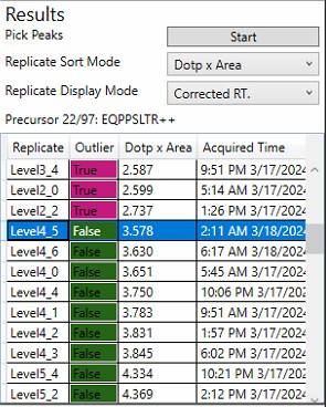
Replicate Sort Mode
- Dotp x Area
- The replicates in the grid and the lower plots are sorted from lowest-to-highest dot product times peak area. This can be useful because this is what Expert Review does when categorizing the replicates.
- Acquire Time
- The replicates in the grid and the lower plots are sorted from lowest-to-highest .raw file acquisition time.
- Dotp x Area
-
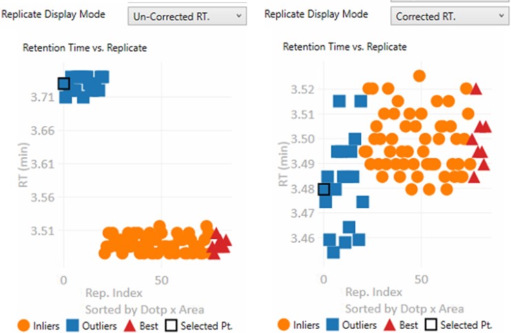
Replicate Display Mode
- Un-corrected RT.
- The retention time graph presents the retention times as they were after the Replicate-Level scoring. These retention times are never sent to Skyline
- Corrected RT.
- These are the retention times after both Replicate-Level and Experiment-Level scoring. These retention times are sent to Skyline when the Send button is pressed.
- These are the retention times after both Replicate-Level and Experiment-Level scoring. These retention times are sent to Skyline when the Send button is pressed.
- Un-corrected RT.
-
Replicate Grid
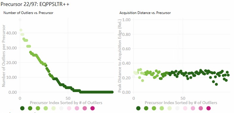
- The currently selected precursor name, and outlier order number is displayed at the top of the grid. The outlier order number is the rank order of this precursor, where #1 has the most outliers that were corrected with Experiment-level scoring, and the last (97 for this assay) has the fewest outliers.
- Clicking any row will sync this precursor and replicate to Skyline, so you can see what the chromatogram looks like. The graphs on the right will be updated to display a black outline around the currently selected replicate.
- If the grid is selected, you can press the Up and Down key to advance the rows.
Skyline
This section is used to send the Expert Review integration boundaries to Skyline.
- Skyline Connection
- This field reports whether the associated Skyline file is open or not. If the Skyline file is closed, then the integration boundaries can no longer be sent to that file
- Send
- Pressing this button causes the calculated integration boundaries from Expert Review to be imported to the associated Skyline document.
Graphs
Clicking on any point is synchronized with Skyline, such that the chromatogram for that precursor is displayed. Clicking on a point will update the lower graphs with the replicate information for that precursor. Pressing the Left or Right key will advance the precursor in that direction.
- Precursor-level graphs
- Number of Outliers
- The left plot displays the sorted number of outliers that were corrected by the Experiment-level scoring for each precursor. The fact that a precursor has many corrected outliers does not necessarily mean that there will be any integration boundary errors in the final output. It does mean that there is some ambiguity though in the data, and it is probably worth investigating the precursors with the most errors.
- Acquisition Distance
- This plot depicts the average relative distance of the peak apex to an edge of an acquisition. For example, if the peak is at 10.4 minutes, and the acquired spectra spanned the range from 10.0 to 12 minutes, then the relative distance would be 0.4 / 2.0.
- It may be worth investigating precursors that have very small acquisition distances to see if there is any truncation of the peaks.
- Number of Outliers
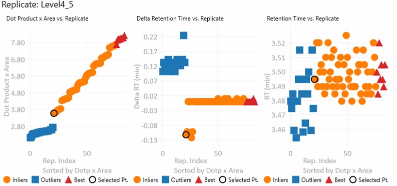
- Replicate-level graphs
These graphs show information for all the replicates for the currently selected precursor.- Dot product x Area
- The dot product is relative to the reference data set. This metric is a way to rank the quality of a replicate.
- The "best" group, in red triangles is determined by this metric.
- Inliers are replicates that aren't in the best group, but did not have their RT updated by Experiment-level scoring.
- Delta Retention Time
- This is the difference between the peak RT. and its average neighbor's peaks RT. This value is likely to be conserved even when there is an absolute RT shift across replicates, and we have investigated using this value for outlier identification and correction.
- Retention Time
- These are the apex retention times of the picked peaks. They can be displayed with the Experiment-level outliers corrected, or uncorrected, depending on the value of Results:Replicate Display Mode.
- These are the apex retention times of the picked peaks. They can be displayed with the Experiment-level outliers corrected, or uncorrected, depending on the value of Results:Replicate Display Mode.
- Dot product x Area
Sequence Import Configure
Sequence Import Configure Reference
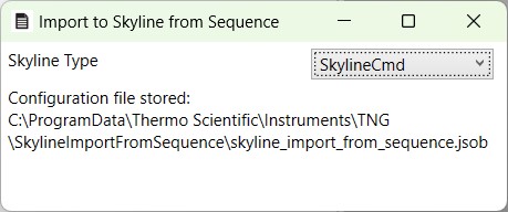
Sequence Import Configure is a tiny application that saves a file on the instrument computer, which allows to automatically import .raw files into a Skyline file after the .raw file acquisition is finished, freeing you from manual File / Import / Result operations.
Steps to configure .raw file import to a Skyline file
-
Run this program. There's no options, just run it. The program finds the SkylineCmd.exe application path, and saves it to a fixed location so that the instrument software can use it to import .raw files.
-
In a future Xcalibur 4.8 release, there will be a native Skyline column, that has a file chooser, and does some simple validation. This column will be accessed by a future Stellar MS software, 1.2.
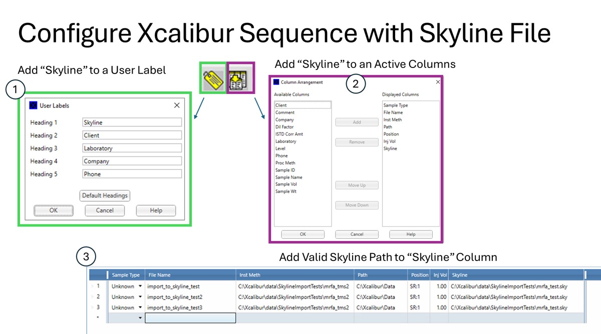
- For Xcalibur < 4.8 and Stellar 1.1 software the following few steps should be taken:
- Add Skyline to an Xcalibur "User Label".
- Configure the new Skyline column by adding it to the Active columns.
- In the Xcalibur sequence, add the full file path to an existing Skyline file, including the .sky extension. For example, D:\MyFiles\skyline_test.sky
That's it!
- The import task has to wait for the LC to finish doing what it's doing, for the .raw file to close and become available for import. This can take a while, even 5-10 minutes, depending on your LC setup and equilibration settings.
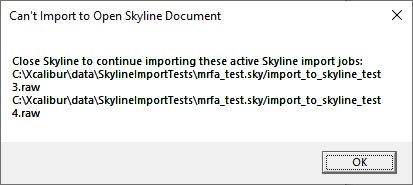
- Note that if you have the Skyline file open when the acquisition ends, we will raise a little dialog telling you that we can't import the .raw files until you close the Skyline file.
- We'll keep a queue of the pending import jobs for up to 72 hours, then we'll give up.
- If you manually imported the .raw file, we will not import it again.