Table of Contents |
guest 2025-07-01 |
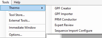
GPF Creator
GPF Importer
PRM Conductor
Expert Review
Sequence Import Configure
PRM Conductor Walkthrough
Absolute Quantitation - PQ500
Neat Unscheduled Runs
Plasma Wide Window Scheduled
Plasma Narrow Windows Scheduled
Label Free - E. Coli
Validation with Subset Replicates
Analysis of Final Assay Replicates
Known Issues
Stack Overflow when Exporting Methods
Hypothesis-driven discovery with Multiple Target Monitoring
Step 1: Pilot experiments with gas phase fractionation
Step 2: Building method with multiple target monitoring
Expert Review Walkthrough
Absolute Quantitation - PQ500
Label Free - E. Coli
Thermo External Tools Overview
Introduction
As of mid-2025, the Thermo set of External tools downloaded under the name PRM Conductor includes 5 different tools
- GPF Creator
- an small application that automates the creation of multiple instrument method DIA files to span a precursor range for a gas-phase-fractionation experiment
- GPF Importer
- a small application that automates the import of GPF or any peptide search data from Proteome Discoverer. This program imports the data with defaults that are appropriate for the Stellar MS, but the same result can be achieved through the Skyline File / Import / Peptide Search wizard.
- PRM Conductor
- an application that aids in the creation of targeted MS methods. This program filters "bad" transitions, and selects "good" peptides via a set of criteria, and helps the user to create one or more instrument methods that will be acquired with at least a required number of points per peak.
- Expert Review
- an application that helps achieve consistent peak integration boundaries, through the use of replicate-level and experiment level correlations to reference data of various types.
- Sequence Import Configure
- a tiny application that saves a file on the instrument computer, which allows to automatically import .raw files into a Skyline file after the .raw file acquisition is finished
GPF Creator
GPF Creator Quick Reference
GPF Creator is small application that automates the creation of multiple instrument method DIA files to span a precursor range for a gas-phase-fractionation experiment.
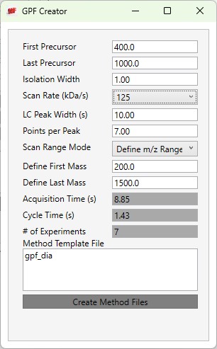
- First Precursor
- The lower bounds precursor m/z
- Last Precursor
- The upper bounds precursor m/z
- Isolation Width
- The quadrupole mass filter isolation width. The precursor range is split up into a series of acquisitions having this stride.
- Scan Rate (kDa/s)
- The ion trap mass analysis rate. This value determines how fast the acquisitions are acquired, and affects the number of experiments needed to span the precursor range.
- LC Peak Width (s)
- The expected LC peak width at the base. The cycle time is this value divided by the desired points per peak.
- Points per Peak
- The minimum acquired points per LC Peak width. The cycle time is the LC peak width divided by this value.
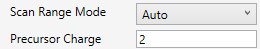
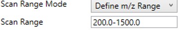
- Scan Range Mode
- Define m/z Range
- Define an explicit first and last mass for the acquired spectra. The acquisition rate is inversely proportional to the size of the m/z range.
- Define m/z Range
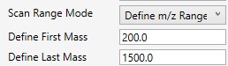
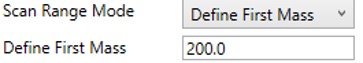
- Define First Mass
- Define a constant first mass for all acquisitions. The last mass is determined based on the charge state, such that last_mass = precursor_mz * charge + 10
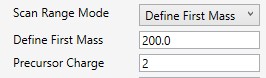
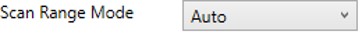
- Auto
- The first and last mass are determined automatically. The last mass is determined as in the Define First Mass mode. The first mass is determined as the lowest mass that still retains most of the ions at the last mass, based on experimental evaluations.
- Acquisition Time(s)
- The total estimated amount of time to acquire data for all the acquisitions from the First Precursor to the Last Precursor, with the given settings. The # of Experiments is this value divided by the Cycle Time, rounded up to the next integer.
- Cycle Time (s)
- The desired cycle time, based on the LC Peak Width / Points per Peak
- Number of Experiments
- The total number of experiments required to span the Precursor range with the current settings. This is the number of instrument methods that will be created when Create Method Files is clicked.
- Method Template File
- Double click this text box to open a file chooser for instrument .meth files. The file should have at least one DIA experiment, not counting Adaptive RT experiments (ART). The first non-ART experiment will be modified in the newly created files. The method should have all the LC details desired, and have the appropriate Method Duration and Experiment Durations.
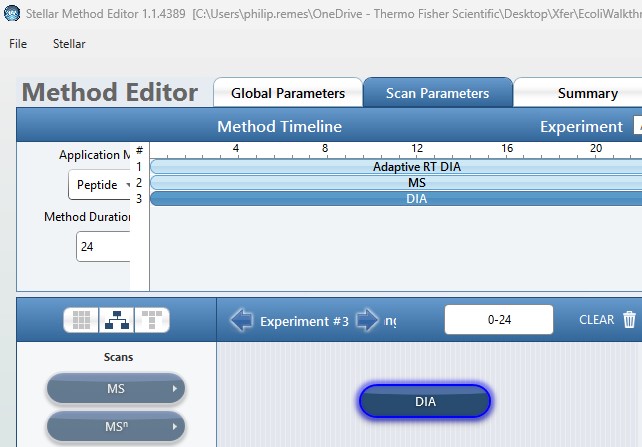
- Create Method Files
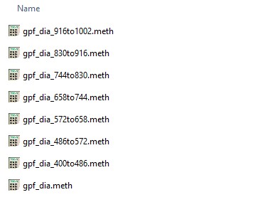
- Click this button to create the instrument methods. Each method will have the name of the template method, with the precursor mass range appended to the end. For example for the gpf_dia.meth template method, files with names like gpf_dia_572to658.meth are created.
GPF Importer
GPF Importer Quick Reference
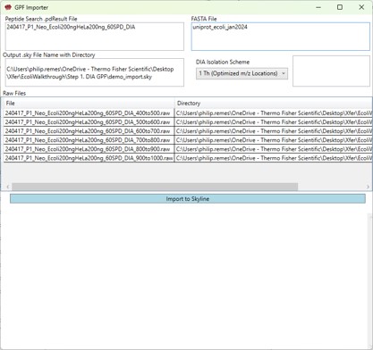
GPF Importer is a small application that automates the import of GPF or any peptide search data from Proteome Discoverer. This program imports the data with defaults that are appropriate for the Stellar MS, but the same result can be achieved through the Skyline File / Import / Peptide Search wizard.
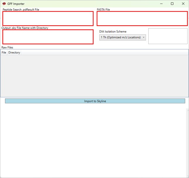
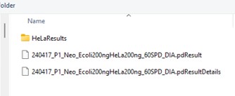
- Peptide Search .pdResult File
- Double click to open a file chooser for a .pdResult file. Since PD v3.1, a corresponding file with the .pdResultDetails extension must be present in the same folder.
-
Fasta File
- Double click to open a file chooser for a .fasta file.
-
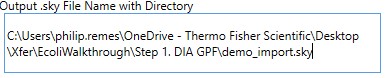
Output .sky File Name with Directory
- Enter the full path to where you want the output .sky file to be. The folder must exist, and the extension of the file must be .sky for the red outline around the box to go away. Usually one can copy the path to a folder and paste here, and then type the desired .sky file.
- Enter the full path to where you want the output .sky file to be. The folder must exist, and the extension of the file must be .sky for the red outline around the box to go away. Usually one can copy the path to a folder and paste here, and then type the desired .sky file.
-
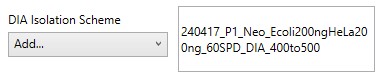
DIA Isolation Scheme
- Select the isolation width used for your experiment. The chooser assumed that you used the Window Placement Optimization option in the Method Editor.
- Select the isolation width used for your experiment. The chooser assumed that you used the Window Placement Optimization option in the Method Editor.
If for some reason, you didn't use Window Placement Optimization in the DIA method, it's possible to select a .raw file that has the DIA isolation scheme that you want to do. This is equivalent to using Skyline to Add an isolation scheme, and selecting Import.
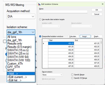
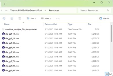
The GPF creator does this for the pre-defined schemes, by creating a short 1 minute instrument method with a scheme, and acquiring the .raw file through Tune. You can find the template raw files if you can find the installed Skyline Tools directory by inspecting the Skyline Immediate Window when you launch a tool.
-
Raw Files
- Double click this box to select one or more .raw files that will be imported to the created .sky file after the spectral library is created from the .pdResult files.
- Double click this box to select one or more .raw files that will be imported to the created .sky file after the spectral library is created from the .pdResult files.
-
Import to Skyline
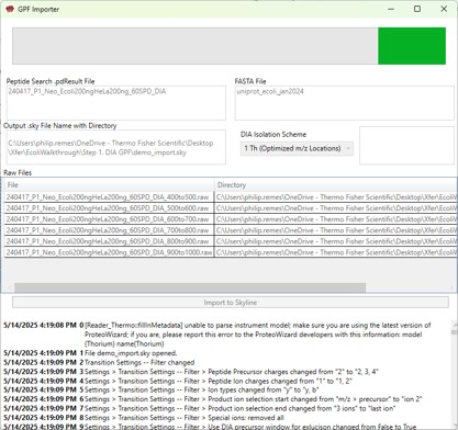
- Click this button to start the import. As the import happens, the Skyline API logging text will print to the lower text box.
- Click this button to start the import. As the import happens, the Skyline API logging text will print to the lower text box.
Once the import is finished (it can take minutes), the output skyline file will open, with all the data imported. You would be ready to create an assay with PRM Conductor next.
PRM Conductor
PRM Conductor Quick Reference
PRM Conductor is an application that aids in the creation of targeted MS methods. This program filters "bad" transitions, and selects "good" peptides via a set of criteria, and helps the user to create one or more instrument methods that will be acquired with at least a required number of points per peak.
Launching PRM Conductor from the Thermo tools menu will open the application. If there was data in the Skyline document, a report will be exported from Skyline and imported to PRM Conductor. The view will look similar to below.
The user parameters are split into 3 sections; Refine Targets, Define Method, and Create Method
Refine Targets
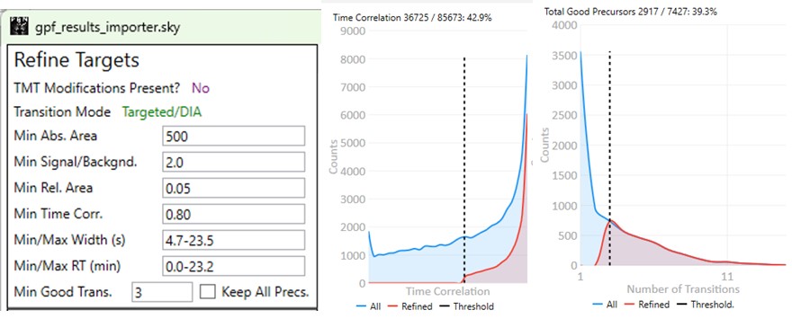
These parameters configure a series of simple filters for the transitions, and allows to filter precursors by the number of good transitions that they have.
- TMT Modifications Present?
- This value is No if there are no TMT modifications. If TMT modifications are present, then the exported methods can account for this, for example by choosing MS3 precursors that have TMT tags.
- Transition Mode
- This value is Precursor/DDA if ALL the analytes have precursor transitions. The 1.0 PRM Conductor version would set this mode if ANY precursor transition was present, which was confusing. This DDA mode means that MS2 data may only be acquired once per LC peak, and so some metrics like Time Correlation are not valid. This mode is common for Small Molecule analysis when data are imported from Compound Discoverer. PRM Conductor is still useful in this case, to create instrument methods, but it may be advisable to select Keep All Precs. option, and apply filtering on a later targeted data set.
- This value is usally Targeted/DIA, enabling the full filtering functionality of the Time Correlation filter.
- Min. Abs. Area
- Filters transitions by requiring that they have a minimum absolute area value. This value may have to change for data acquired on different instruments. For example, the intensity scaling on Orbitrap instruments is arbitrarily scaled to a value that is ~10x the value for Ion trap and Astral data.
- Min. Signal / Backgnd.
- Filters transitions by requiring that they have a minimum signal to background ratio. Signal is the Skyline peak area, and Background is the Skyline background value. This value should be used sparingly, because the current background metric that we use is not as good as it could be.
- Min. Rel. Area
- Filters transitions by requiring that they have a minimum relative area to the largest transition for its precursor.
- Min. Time Corr.
- Filters transitions by requiring that they have a minimum correlation to the median transition. This value is called Shape Correlation by Skyline,and was defined by Searle et. al., and later in some detail by Heil et. al.
- Min./Max. Width (s)
- Filters transitions by requiring that their base LC width be within the given bounds. The bounds is computed from the Skyline FWHM and converted to a base peak width by assuming a Gaussian shape and multiplying by 2.54. See the supplement of Remes et. al. for a derivation.
- Min./Max. RT (min)
- Filters precursors by requiring that their retention time be within the given bounds.
- Min. Good Transitions
- Filters precursors by requiring at least this many transitions that satisfy the above filters.
- Keep All Precs.
- This option ensures that no precursors are filtered, and the top Min. Good Transitions are kept. If there are not enough good transitions, "bad" transitions are selected according to Area x Time Corr. This option is useful when the user wants to keep all the precursors and just clean up the transitions, or is using DDA mode.
Define Method
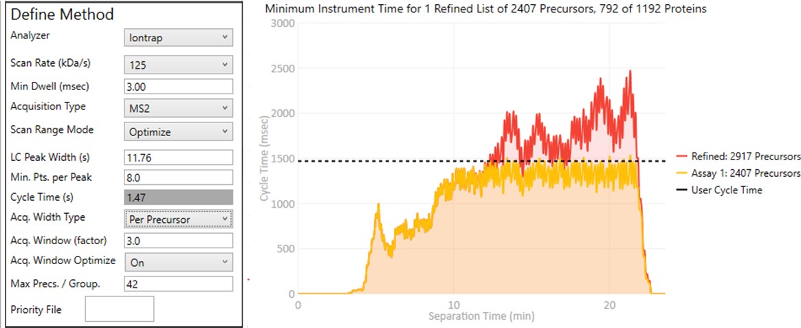
These parameters control how many targets can be included in the assay. When parameters in this section are changed, and the 'enter' key is pressed, the graph on the right will update, showing how many precursors can be included in the assay, while respecting Cycle Time defined by the LC Peak Width and the Min. Pts. per Peak.
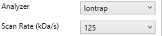
Analyzer
- Ion Trap
- Scan Rate (kDa/s)
- Sets the analysis scan rate. This value affects the acquisition rate, and therefore the assay target capacity.
- Scan Rate (kDa/s)
-
Astral
- Currently the Astral has no analyzer-specific parameters
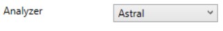
- Currently the Astral has no analyzer-specific parameters
-
Orbitrap
- Resolution (k)
- Sets the analysis resolution. This value affects the acquisition rate, and therefore the assay target capacity.
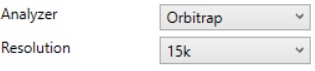
- Sets the analysis resolution. This value affects the acquisition rate, and therefore the assay target capacity.
- Resolution (k)
-
Triple
- Max #Transitions
- Only up to this number of transitions will be selected, since this value linearly decreases the assay target capacity.
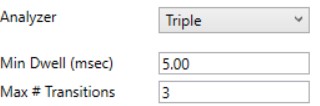
- Only up to this number of transitions will be selected, since this value linearly decreases the assay target capacity.
- Max #Transitions
-
Min Dwell (msec)
- Also called injection time on many instruments, this value sets the smallest amount of precursor accumulation time per target. Typically we set this value small enough so that it does not affect the assay capacity, and rely on the dynamic AGC algorithm to boost the injection time according to the available time in the cycle. See Remes et. al. for a description of the dynamic AGC process.
- In some cases, the experimenter may know that to achieve high quality data, a minimum dwell time is needed, and will adjust this value accordingly.
Acquisition Type
- MS2
- The standard analysis type, where each acquisition contains data for a single precursor that is mass selected and fragmented.
- MS3
- Currently only available when Ion Trap analyzer is selected, in this mode, each acquisition contains data for a single precursor that is mass selected, fragmented, and one or more fragments are further mass selected and fragmented.
- The Max # Transitions parameter becomes available in this mode, limiting the number of MS3 precursors that will be simultaneous mass analyzed in the second MS stage. For purposes of the acquisition rate estimations, this mode currently assumes that resonance CID with 4 msec activation time is used for the first activation, and HCD is used for the second activation. In reality if the user selects a method template the uses resonance CID for the second activation, then the activation for each MS3 precursor is performed serially, taking at least #transitions x activation_time to be performed.
-
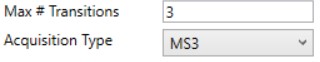
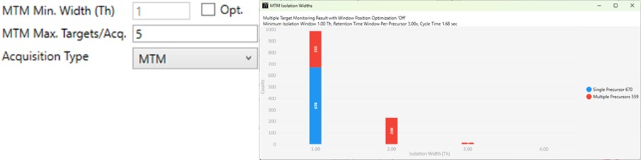
MTM
- Multiple target monitoring is a type of method that can be generated from 1 Th isolation window GPF DIA data. It analyzes the GPF data to determine when it is safe to expand the number of targets, or the isolation width, to encompass multiple targets. MTM can be used to expand the number of targets in an assay compared to normal PRM, or alternatively for the same number of targets, MTM can enable the use faster gradients and higher throughput, or higher injection times and better sensitivity.
- When the Opt. check box is unchecked, then the isolation widths are multiples of the GPF isolation width, which is shown in a disabled text box (1 here). A pop-up window shows the distribution of isolation widths, and how many of them are for single or multiple targets.
- When the Opt. check box is checked, then the isolation widths are customized for each acquisition, such that the window size is (largest_mz - smallest_mz) + MTM Min. Width (Th).
-
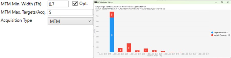
DDIA
- Dynamic DIA is a type of DIA method in which the precursor range shifts as a function of the experiment time. This method can be used to acquire data with a narrower isolation window than would be possible if data for the entire precursor range had to acquired on each cycle.
- The DDIA Width(Th) sets the isolation width that will be used. Narrower widths will acquire higher quality data, for fewer precursors.
- A pop-up plot appears that shows the density of precursors in the Skyline document, along with lines that trace the proposed precursor range as a function of experiment time.
Scan Range Mode
-
Define m/z Range
- Define an explicit first and last mass for the acquired spectra. The acquisition rate is inversely proportional to the size of the m/z range.
- Define an explicit first and last mass for the acquired spectra. The acquisition rate is inversely proportional to the size of the m/z range.
-
Define First Mass
- Define a constant first mass for all acquisitions. The last mass is determined based on the charge state, such that last_mass = precursor_mz * charge + 10
- Define a constant first mass for all acquisitions. The last mass is determined based on the charge state, such that last_mass = precursor_mz * charge + 10
-
Auto
- The first and last mass are determined automatically. The last mass is determined as in the Define First Mass mode. The first mass is determined as the lowest mass that still retains most of the ions at the last mass, based on experimental evaluations.
- The first and last mass are determined automatically. The last mass is determined as in the Define First Mass mode. The first mass is determined as the lowest mass that still retains most of the ions at the last mass, based on experimental evaluations.
-
Optimize
- The first and last mass are set based on the set of "good" transitions for a precursor plus a small buffer. This mode enables the fastest acquisition rates possible for the Ion trap analysis, where the mass analysis time is directly proportional to the scan range.
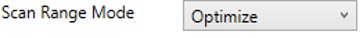
- The first and last mass are set based on the set of "good" transitions for a precursor plus a small buffer. This mode enables the fastest acquisition rates possible for the Ion trap analysis, where the mass analysis time is directly proportional to the scan range.
Other Define Method Parameters
-
LC Peak Width (s)
- The expected LC peak width at the base. This value is pre-populated from the input data, but can be updated as desired. The instrument maximum cycle time is this value divided by the desired points per peak.
-
Points per Peak
- The minimum desired acquisition points per LC Peak width. The cycle time is the LC peak width divided by this value.
-
Cycle Time (s)
- The desired cycle time, based on the LC Peak Width / Points per Peak
-
Acquisition Width Type
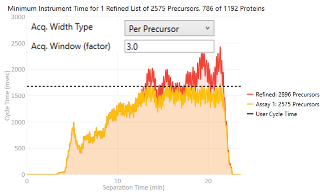
Defines the method used to set the acquisition window width around each target in the method.- Global
- All targets get the same, global acquisition window size, Acq. Window (min).

- All targets get the same, global acquisition window size, Acq. Window (min).
- Per precursor
Each target gets an acquisition window width defined as its individual base peak width, times the Acq. Window (factor) value.
- Global
-
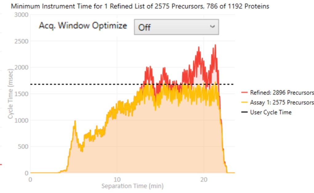
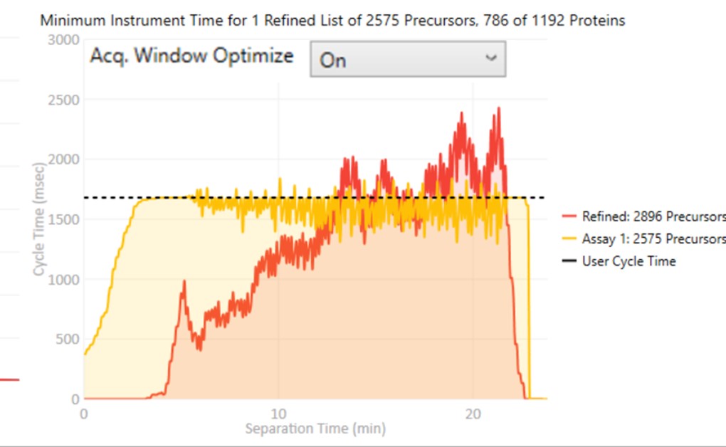
Acq. Window Optimize
- When set to Off, the acquisition windows will be exactly the ones determined based on the current Acquisition Width Type. Note how the Assay 1 density in yellow is the same as the Refined density in red in the time region from 0 to ~10 minutes.
- When set to On, then the acquisition windows widths are expanded by up to some factor (5x currently), while ensuring that the acquisitions don't exceed the desired cycle time. Note how the Assay 1 density matches the cycle time for much of the region between 0 and 10 minutes now. The reason for this mode is that early eluting molecules can have variable retention times, and Adaptive RT may have little information to be able to adjust the targeted schedule at these early times. Making the widths larger in a dynamic way is a nice way to make the assay acquisition more robust. In the future we could add a UI parameter that specifies the maximum expansion factor.
- When set to Off, the acquisition windows will be exactly the ones determined based on the current Acquisition Width Type. Note how the Assay 1 density in yellow is the same as the Refined density in red in the time region from 0 to ~10 minutes.
-
Max Precs. / Group
- Sets the maximum number of peptides per protein in Skyline's Peptide mode, or molecules per molecule group in Skyline's Molecule mode. This parameter can be used to increase assay quality by removing targets from the assay that may not add additional information. The included targets are selected by their quality, defined as their Area x Time Correlation.
-
Priority File
- Double click to select a file with a .prot extension that you've made. Just create a text file, and save it with the .prot extension. On each line, you can enter a protein name, or molecule list name. Skyline puts either the protein name or molecule list name in the Report column called "Molecule List". Any precursors that belong to the protein or molecule list will be accepted into the assay, even if they don't pass all the filters.
- Using a Priority file is a good way to incorporate iRT compounds into an assay, when doing an initial search for heavy-labeled standards.
- If the Balance Load check box is not checked, then each of the multiple assays that may be generated will contain the prioritized targets.
- New for v1.1, you can also enter peptide sequences or molecule names. These are the values found in the Skyline report columns called, "Modified Sequence Monoisotopic Masses", or "Molecule", in the Skyline Protein or Molecule modes, respectively.
- For example, the file could have 2 peptide sequences and a protein name.
LPALFC[+57.021464]FPQILQHR
ESYGYNGDYFLVYPIK
SPEA_ECOLI
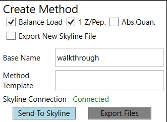
Create Method
These parameters control aspects of how the method will be created.
-
Balance Load
- When checked, a single assay will be created that respects the currently defined Cycle Time. The number of Refined precursors added will depend on the particular choice of Define Method parameters. Precursors are added to the assay iteratively from each protein or molecule group in turn, where the precursors from each group are added in order from highest to lowest quality. Quality is currently defined as area x time correlation. A balanced load refers to how the precursor time density becomes uniform at the limit of many potential precursors, instead of peaked in the middle of the run.
- When not checked, multiple assays will be created that analyze all Refined precursors. Each assay will be of the traditional, non-balanced type. If a Priority File is specified, prioritized precursors will be added to all of the assays.
-
1 Z/Pep.
- When checked, only a single precursor from each peptide (or molecule, in Skyline's Molecule mode) will be accepted into the assay. The selected precursor will have the highest quality, defined as area x time correlation.
- When not checked, multiple precursors having different charge states could be in the assay, if they all passed the various filters.
-
Abs. Quan.
- When checked, a light-version of each heavy-labeled peptide will be added to the assay. This is a nice way to create a light+heavy assay from an initial heavy-only assay. The instrument time plot will update to have 2x the number of targets, allowing to visualize whether enough points per peak will be acquired.
-
Export Skyline File
- When checked, a new Skyline file having the precursors with their corresponding filtered transitions will be created when the Export Files button is pressed. Because creating the new Skyline file takes some 10's of seconds, it can be annoying, and it was made into an option. The good part about using this option is that the new Skyline file will have its Transition Settings set to PRM with Stellar-specific parameters.
- When not checked, no new Skyline file will be created when the Export Files button is pressed. Often we use this mode, and rely on using the Sync to Skyline button to update the current Skyline document, and later save a new Skyline document manually.
-
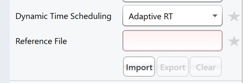
Combine DIA Windows for Reference
- This is a special option that only appears if the input data are DIA with isolation width less than 15 Th, and no large window Adaptive RT information is available.
- When checked, and if the .meth has specified Adaptive RT for Dynamic Time Scheduling, then the exported method will have an rtbin file that is made by combining acquisitions in silico. The DIA alignment acquisitions will have an isolation width of near 50 Th, and will adjust the target schedule accordingly.
- This is a nice option when creating Stellar MS targeted assays from Astral DIA data, which are likely acquired with small isolation widths, such as 2, 3, or 4 Th.

-
Base Name
- Output files will have this value in them. For example, the .meth, .sky, and .csv files associated with a method will all have use this name.
-
Method Template
- Double click this text box to open a file chooser for a .meth file that will serve as a template for exported assay files. The template file should have a tMSn method in it, and the appropriate LC parameters, and Method and Experiment durations. Other parameters like activation type should also be specified. If Adaptive RT is specified in the Dynamic Time Scheduling, then an rtbin file will be created during export and saved in the .meth file. This is the preferred way to add Adaptive RT functionality to a method.
- You can make methods on your non-instrument computer if you have downloaded the Workstation version of the instrument software. This software is available at the Thermo Flexnet site.
- In this case, you can use the standalone method editor found at C:\Program Files\Thermo Scientific\Instruments\TNG\Stellar\1.1\System\Programs\TNGMethodEditor.exe.
- The standalone method editor only has access to MS information, not the LC driver information, but you can copy a .meth file from an instrument that has the LC information in it, and then resave and modify it on your laptop.
-
Sync to Skyline
- Pressing this button updates the current Skyline file by filtering the transitions, precursors, and proteins that are not in the final assay.
-
Export Files
- Pressing this button will export precursor lists, transitions lists, .meth files if specified in the Method Template field, and a .sky file if Export to Skyline is checked.
Expert Review
Expert Review Quick Reference
Expert Review is an application that helps achieve consistent peak integration boundaries, through the use of replicate-level and experiment level correlations to reference data of various types.
Input
These parameters change how the calculations will be performed. They take affect once the Results:Start button is pushed.
- Isotope Label
Determines whether a specific isotopically-labeled version of the precursor is used for setting the boundaries. Skyline's Isotope Label Type report column is used as input data.- Not Specified
- The isotope label type is not considered. Use this mode for label-free experiments. If this mode is used for data with light and heavy labels, the boundaries that are actually used could come from either molecule (not recommended).
- Heavy
- The integration boundaries from the heavy labeled precursors will be sent to Skyline.
- Light
- The integration boundaries from the endogenous, or light, precursors will be sent to Skyline.
- Not Specified
- Use Other Label's Info
- This parameter is only visible if the Isotope Label parameter is set to Light or Heavy.
- On
- Experiment-level replicate analysis will use information from the other label when attempting to place consistent integration boundaries. Ex. information from the light precursor is used to help determine the heavy precursor boundaries.
- We recommend to use "On", but include this option in case the light data are not consistent between replicates and are hampering the boundary location accuracy.
- Off
- Experiment-level replicate analysis will not use information from the other labeled precursor.
- Impute RT Outliers
- On
- Uses a local regression analysis of retention time and raw file acquisition time to attempt to identify and correct retention time outliers.
- This algorithm is applied after the cross-corrleation based experiment-level replicate analysis.
- This algorithm uses information from the retention times and acquisition times "best" replicates. If these best replicates are all acquired at the start of an experiment, and there is later significant RT drift, the algorithm is not very accurate.
- This algorithm can be useful if there are retention time drifts that vary smoothly with acquisition time. Only use this mode if there are no abrupt shifts in retention time between replicates. Such shifts will cause this algorithm issues.
- Off
- No local regression analysis of retention time and raw file acquisition time is used. The cross correlation-based experiment-level analysis is still used, however.
- On
- Reference File
Expert Review relies on information from a reference replicate or replicates to perform integration boundary determination. The reference can be currently be selected in two ways.- Current
- Select this button to update the Replicates grid with information from the current Skyline file.
- Select
- This button will open a file chooser, whereupon the user can choose another Skyline file to use as a reference. This can allow for faster processing, since the reference data can be smaller and load faster. The only gotcha is that if your reference file transitions for some reason don't overlap with the experiment transitions, or there were precursors in the experiment file that aren't in the reference file, there would be an error.
- Current
- Reference File Text Box
- The current reference Skyline file is displayed here. Note that for convenience, Expert Review remembers your last choice of reference Skyline file. This can get you into trouble when you use Expert Review for a new experiment, and you have the old reference specified.
- Reference File Replicate Grid
- The replicates for the reference Skyline file are displayed. For files with multiple replicates, you can select which one or more replicates to use as reference.
- Multiple replicates might make sense in a multi-injection replicate scenario, where all the precursors are spread amonst replicates.
- If you selected multiple replicates, and the same precursor is in both replicates, the replicate information that is actually used is not well defined.
- The replicates for the reference Skyline file are displayed. For files with multiple replicates, you can select which one or more replicates to use as reference.
Results
These parameters are for starting the processing, or perusing the results.
-
Pick Peaks
- Press this button once the Input parameters have been set. The processing will start, which could take some time, depending on the size of the Skyline file. For many experiments, it takes less than a minute. The largest Skyline file we tried ha 1000 replicates for 83 precursors. It took 40 minutes for Skyline to export the report, and 5 minutes to determine the integration boundaries.
- After the processing finishes, the selected precursor in Skyline becomes the one with the most outliers that were corrected with Experiment-level scoring. If this gets annoying for users, we can remove this feature.
-
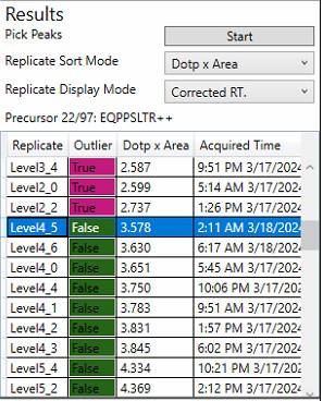
Replicate Sort Mode
- Dotp x Area
- The replicates in the grid and the lower plots are sorted from lowest-to-highest dot product times peak area. This can be useful because this is what Expert Review does when categorizing the replicates.
- Acquire Time
- The replicates in the grid and the lower plots are sorted from lowest-to-highest .raw file acquisition time.
- Dotp x Area
-
Replicate Display Mode
- Un-corrected RT.
- The retention time graph presents the retention times as they were after the Replicate-Level scoring. These retention times are never sent to Skyline
- Corrected RT.
- These are the retention times after both Replicate-Level and Experiment-Level scoring. These retention times are sent to Skyline when the Send button is pressed.
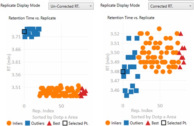
- These are the retention times after both Replicate-Level and Experiment-Level scoring. These retention times are sent to Skyline when the Send button is pressed.
- Un-corrected RT.
-
Replicate Grid
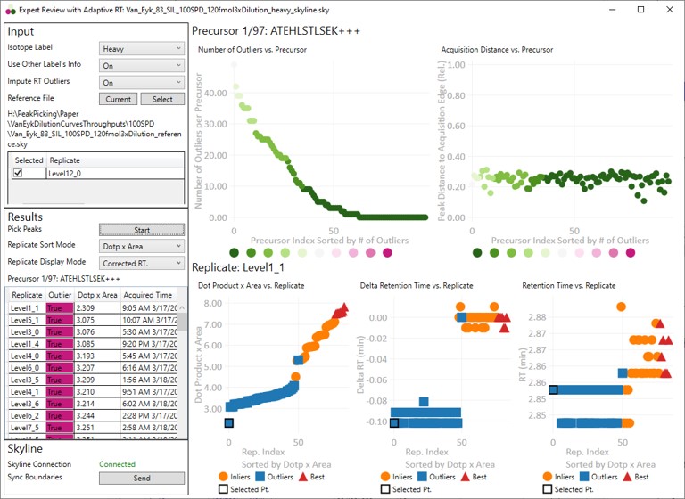
- The currently selected precursor name, and outlier order number is displayed at the top of the grid. The outlier order number is the rank order of this precursor, where #1 has the most outliers that were corrected with Experiment-level scoring, and the last (97 for this assay) has the fewest outliers.
- Clicking any row will sync this precursor and replicate to Skyline, so you can see what the chromatogram looks like. The graphs on the right will be updated to display a black outline around the currently selected replicate.
- If the grid is selected, you can press the Up and Down key to advance the rows.
Skyline
This section is used to send the Expert Review integration boundaries to Skyline.
- Skyline Connection
- This field reports whether the associated Skyline file is open or not. If the Skyline file is closed, then the integration boundaries can no longer be sent to that file
- Send
- Pressing this button causes the calculated integration boundaries from Expert Review to be imported to the associated Skyline document.
Graphs
Clicking on any point is synchronized with Skyline, such that the chromatogram for that precursor is displayed. Clicking on a point will update the lower graphs with the replicate information for that precursor. Pressing the Left or Right key will advance the precursor in that direction.
- Precursor-level graphs
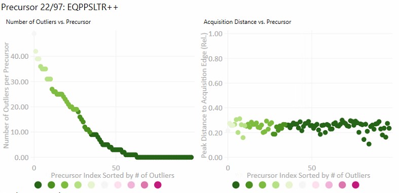
- Number of Outliers
- The left plot displays the sorted number of outliers that were corrected by the Experiment-level scoring for each precursor. The fact that a precursor has many corrected outliers does not necessarily mean that there will be any integration boundary errors in the final output. It does mean that there is some ambiguity though in the data, and it is probably worth investigating the precursors with the most errors.
- Acquisition Distance
- This plot depicts the average relative distance of the peak apex to an edge of an acquisition. For example, if the peak is at 10.4 minutes, and the acquired spectra spanned the range from 10.0 to 12 minutes, then the relative distance would be 0.4 / 2.0.
- It may be worth investigating precursors that have very small acquisition distances to see if there is any truncation of the peaks.
- Number of Outliers
- Replicate-level graphs
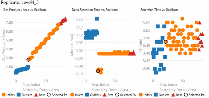
These graphs show information for all the replicates for the currently selected precursor.- Dot product x Area
- The dot product is relative to the reference data set. This metric is a way to rank the quality of a replicate.
- The "best" group, in red triangles is determined by this metric.
- Inliers are replicates that aren't in the best group, but did not have their RT updated by Experiment-level scoring.
- Delta Retention Time
- This is the difference between the peak RT. and its average neighbor's peaks RT. This value is likely to be conserved even when there is an absolute RT shift across replicates, and we have investigated using this value for outlier identification and correction.
- Retention Time
- These are the apex retention times of the picked peaks. They can be displayed with the Experiment-level outliers corrected, or uncorrected, depending on the value of Results:Replicate Display Mode.
- These are the apex retention times of the picked peaks. They can be displayed with the Experiment-level outliers corrected, or uncorrected, depending on the value of Results:Replicate Display Mode.
- Dot product x Area
Sequence Import Configure
Sequence Import Configure Reference
Sequence Import Configure is a tiny application that saves a file on the instrument computer, which allows to automatically import .raw files into a Skyline file after the .raw file acquisition is finished, freeing you from manual File / Import / Result operations.
Steps to configure .raw file import to a Skyline file
-
Run this program. There's no options, just run it. The program finds the SkylineCmd.exe application path, and saves it to a fixed location so that the instrument software can use it to import .raw files.
-
In a future Xcalibur 4.8 release, there will be a native Skyline column, that has a file chooser, and does some simple validation. This column will be accessed by a future Stellar MS software, 1.2.
- For Xcalibur < 4.8 and Stellar 1.1 software the following few steps should be taken:
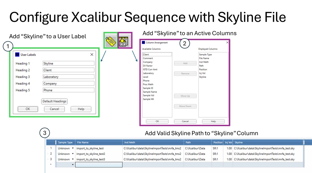
- Add Skyline to an Xcalibur "User Label".
- Configure the new Skyline column by adding it to the Active columns.
- In the Xcalibur sequence, add the full file path to an existing Skyline file, including the .sky extension. For example, D:\MyFiles\skyline_test.sky
That's it!
- The import task has to wait for the LC to finish doing what it's doing, for the .raw file to close and become available for import. This can take a while, even 5-10 minutes, depending on your LC setup and equilibration settings.
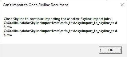
- Note that if you have the Skyline file open when the acquisition ends, we will raise a little dialog telling you that we can't import the .raw files until you close the Skyline file.
- We'll keep a queue of the pending import jobs for up to 72 hours, then we'll give up.
- If you manually imported the .raw file, we will not import it again.
PRM Conductor Walkthrough
PRM Conductor Introduction
PRM Conductor is a software program that plugs into the Skyline External Tool ecosystem. The purpose of PRM Conductor is to aid in the creation of parallel reaction monitoring (PRM) mass spectrometry methods. The basic functions of the program are as follows:
- Receive DIA or PRM data
- Filter transitions with a set of filters
- Filter precursors that have at least N good transitions
- Visualize the scheduling of one or more PRM assays with particular acquisition parameters
- Export an instrument method for the new assay(s)
- Support the setup of the Adaptive RT algorithm for real-time chromatogram alignment
Location of the Walkthrough Materials
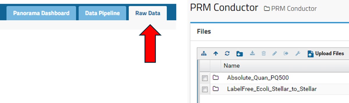
All the documents needed to perform the walkthroughs can be found by clicking the Raw Data tab on the top right hand side of this page.
Example Scenario
PRM Conductor is launched from Tools / Thermo / PRM Conductor. In one test case, we imported DIA data containing more than 5000 unique peptide identifications.
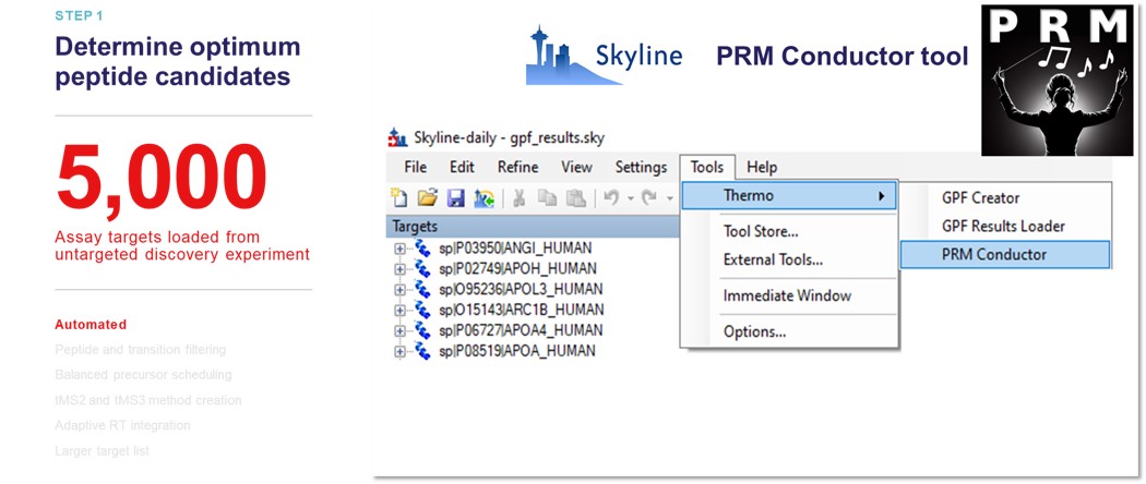
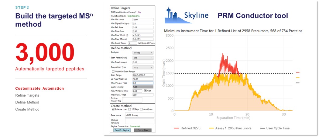
After applying the transition filters listed in the Refine Targets section, there were about 3000 'good' precursors left. The user can alter parameters in the Define Method, such as the Analyzer type, the minimum points per LC peak, and the scheduled acquisition window, and see how the 'good' precursors fit into a scheduled assay. The yellow trace shows precursors that can be acquired in less than the cycle time, while the red trace shows those precursors that can't be acquired. The user can then export a method with the Create Method section, where they can specify an instrument method template with LC details, which will be used to create a new method with the acquisition settings and precursor list filled in.
Walk-throughs
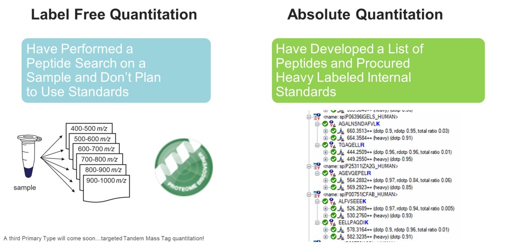
Several walk-throughs have been created to teach users how to make targeted methods with PRM Conductor. These methods generally fall into two categories at present; the absolute quantitation category, where there are heavy standards created for each endogenous peptide to be monitored, and the label-free category, where the assay is created directly from peptide search results, and there are no heavy standards.
Available Walk-throughs
- Absolute Quantitation
- PQ500
- Label Free
- E. coli in HeLa
- Hypothesis-driven Discovery with Multiple Target Monitoring
Absolute Quantitation - PQ500
Biognosys PQ500 Introduction
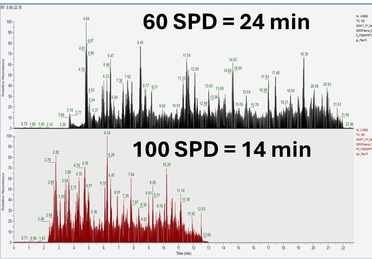
This tutorial will show you how to create a targeted MS2 assay that uses heavy standards for absolute quantitation. The Biognosys PQ500 standard is used as the source of heavy standards. We used the Vanquish Neo LC, ES906A column and a trap-and-elute injection scheme with a 60 SPD method and a 100 SPD method. The gradients have been designed so that compounds elute over a large portion of the experiment spans.
Setting up the Skyline Document
Pierce retention time calibration mixture (PRTC) is used here to create an indexed retention time (iRT) calculator. Along with a spectral library, the iRT calculator will aid Skyline in picking the correct LC peaks in the steps that follow. See the Skyline iRT tutorial for more details. Here we will use an iRT calculator created with Koina. After setting up the LC and column, we run unscheduled PRTC injections to ensure that the LC and MS system is stable. The method file 60SPD_PRTC_Unscheduled.meth can be used for this. The prtc_unscheduled.csv file could be used to import into a tMSn table if making a method from scratch. We like to use Auto QC with Panorama to store all our files, and to automatically upload and visualize QC data.
Now we will create a Skyline document for analyzing PQ500 heavy labeled peptides. Biognosys supplies a transition list with intensities and iRT values that can be used to create a spectral library and iRT calculator. We'll show you though also how you can use use Koina integration with Skyline to create a spectral library and iRT library from a list of peptides sequences if you don't know anything about them. We also tend to like to use Koina spectral libraries even if supplied lists of transitions, because we will be using PRM Conductor to automatically filter the transitions. At the end of this section, we’ll be ready to perform unscheduled PRM for the PQ500 heavy-labeled peptide standards.
Transition Settings
Open up Skyline Daily and create a new document. Save the document as Step 1. Setup Skyline Documents/pq500_60spd_neat_multireplicate.sky.
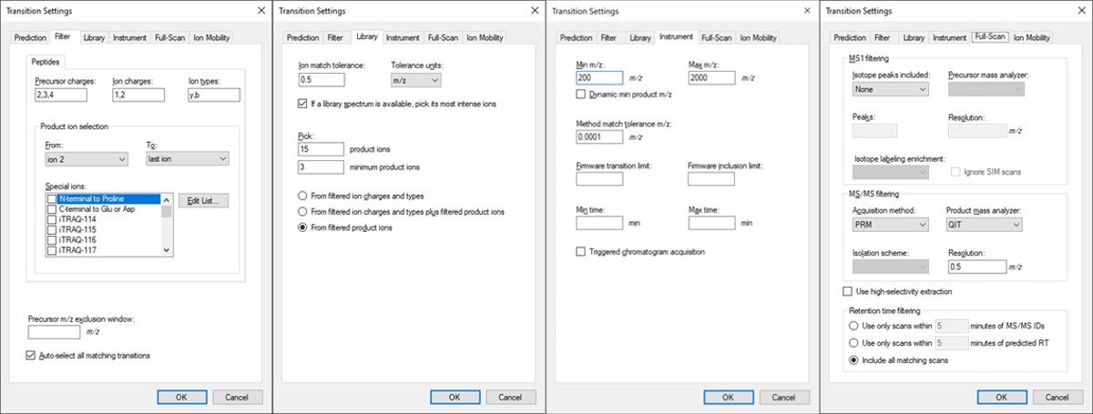
- Open Settings / Transition Settings / Filter. Set Precursor charges to ‘2,3,4’, Ion Charges to ‘1,2’, and Ion types to ‘y,b’. In the Product ion selection section, select ‘From ion 2’ to ‘last ion’. Un-select N-terminal to Proline and keep “Auto-select all matching transitions” checked.
- In the Library tab, set Ion match tolerance 0.5, check the box “If a library spectrum…”, set Pick 15 product ions with minimum 3 product ions. 15 is a large number, but we will refine the transitions later with the PRM Conductor tool. Select “From filtered product ions”.
- In the Instrument tab, set Min m/z 200, and Max m/z 2000. Set the Method match tolerance m/z to 0.0001. This helps Skyline to differentiate between precursors that have very close m/z. As we’ll see later, there are sometimes still peptides with different sequences but the same exact m/z.
- In the Full-Scan tab, set MS1 filtering / Isotope peaks included to None. If there are any precursor transitions, PRM Conductor will think that the document is in DDA mode, and will not be full featured. Set MS/MS filtering / Acquisition Method to PRM, Product mass analyzer to QIT, and Resolution to 0.5 m/z. Set Retention time filtering to Include all matching scans. Press Okay to close the Transition Settings.
Peptide Settings
Open Settings / Peptide Settings.
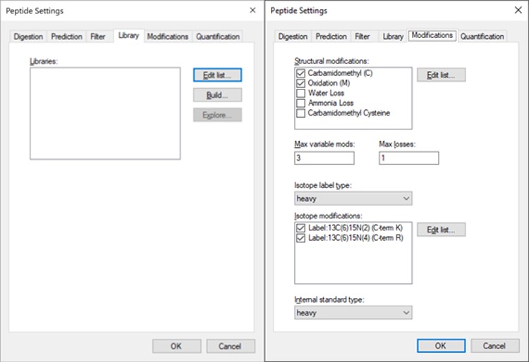
- In the Library tab, uncheck or remove any libraries that are there, for simplicity's sake.
- In the Modifications tab, make sure that Carbamidomethyl (Cysteine) and Oxidation (Methionine) modifications are enabled. The C-term R and C-term K isotope modifications should be enabled. Isotope label type and Internal standard type should be set to heavy.
iRT Calculator from PRTC
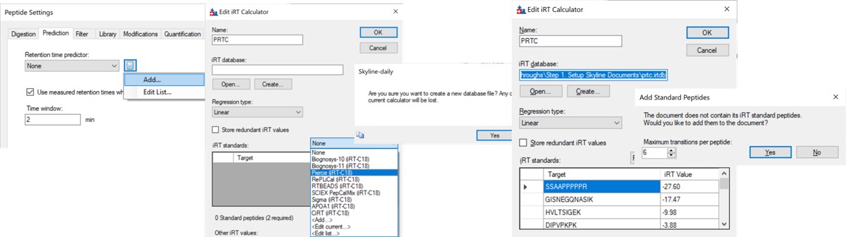
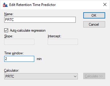
- In the Prediction tab, select the calculator icon and press Add. Add a name like PRTC. In the iRT Standards drop-down menu, select Pierce (iRT-C18). Press the Create button, and select Yes when asked if you want to create a new database file. Give the file a name like prtc.irtdb. Press Okay.
- Go back into the Peptide Settings / Prediction tab, click the dropdown arrow and select Edit current. Set the window to 2 minutes, and press Okay.
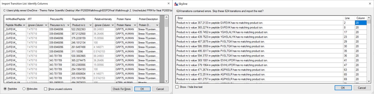
Importing the Transition List
Use File / Import / Transition List and select the file Step 1. Setup Skyline Documents/biognosis_pq500_transition_list.csv. A dialog opens that shows the mapping of the file headers to Skyline variable names. Press Okay to continue on. A new dialog prompts us that 624 transitions are not recognized. These are water losses that we don't necessarily need. We could define water loss transitions in the Settings tabs if we really wanted them. Press Okay twice to exit the iRT calculator dialogs. A new dialog will ask if you want to add the Standard Peptides, choose 6 transitions and press Yes.
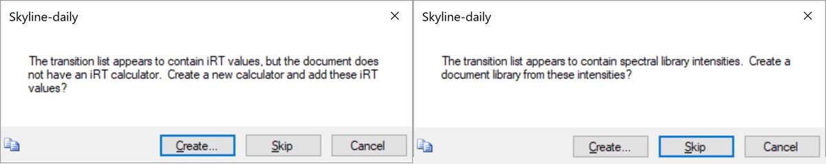
Another dialog appears, asking if we want to make an iRT calculator. The Biognosys values are presumably based on experiment, and are slightly more accurate than the in silico predicted iRT values from Koina, so Click Create. You'll be asked if you want to create a spectral library from the intensities in the transition list. Feel free to press Create if you want, but we will press Skip and use Koina to predict the intensities next. The Skyline document will update and in the bottom right border will be displayed 579 prot, 818 pep, 1622 prec, 9020 tran.
Koina
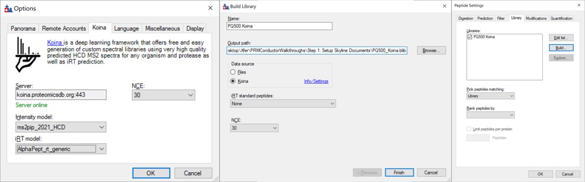
Now we’ll generate a spectral library with Koina.
- Open Tools / Options and go to the Koina tab. Set the intensity model to ms2pip_2021_HCD, the iRT model to AlphaPept_rt_generic, and NCE to 30. Note that our original assay was created when this option tab said Prosit, but it had changed in a new Skyline Daily release by the time that this walkthrough was created. Press Okay.
- Go to Settings / Peptide Settings / Library / Create and select Data source Koina, NCE 30, and set a name and output path for the library. Press Finish. Make sure the library is selected in Peptide Settings Library and press Okay. If everything works correctly and you have internet access, your computer will communicate with the Koina server and return the spectral library to you, and the peptides in the Skyline tree will receive little spectra images to the left of the sequences, like below.
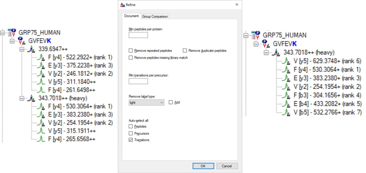
- Open Refine / Advanced and select Remove label type light, and click the box for Auto-select all Transitions, and press Okay. If you expand a peptide, like the first one, GVFEVK, it will have up to 15 transitions, instead of the up to 6 in the Biognosys transition file. Save the Skyline document. This is the end of Step 1: Setting up the Skyline Document.
Neat Unscheduled Runs
- Unscheduled PRM for Neat Heavy PQ500 with Multiple Replicates
Unscheduled PRM for Neat Heavy PQ500 with Multiple Replicates
In this step, we’ll use Skyline to create a set of unscheduled PRM methods for the 804 PQ500 peptides. At the end of this step, we will have created 10 Unscheduled PRM methods for both 60 and 100 SPD, acquired data for them, loaded the results into Skyline, and assessed the results. We’ll be ready to look at our standards spiked into matrix in the next step.
Alternative DIA GPF Acquisition
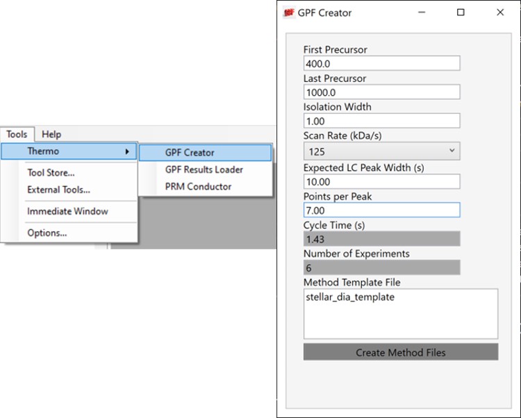
Alternatively, especially as the number of heavy peptides increases, one could opt to use data independent acquisition (DIA) of the neat, heavy standards to find their retention times. One would simply find the smallest and largest m/z of the peptides in question and use the Thermo method editor to create a DIA method. For example, we have had success in some neat standard cases using a single injection with 4 Th isolation width. However multiple gas-phase fractions (GPF) could be acquired with narrower isolation widths, as in the technique we use for identification of unknowns. We included a little helper application in our Thermo suite of external tools called GPF creator that spawns GPF instrument methods. Given a set of parameters, namely a precursor m/z range and a Stellar DIA method template, it will create a cloned set of methods with the appropriate Precursor m/z range filled in. In the case below with Precursor m/z range 400-1000 and 6 experiments, methods would be created for the ranges 400-500, 500-600, all the way to 900-1000. The resulting .raw files could be used in the much the same way that we’ll use the unscheduled PRM data files in the coming steps, only that we would have to configure the Skyline Transition / Full Scan / Acquisition to DIA with the appropriate window scheme (Ex. 400 to 1000 by 1 with Window Optimization On). As it is, we continue on, using the Unscheduled PRM technique.
Creating Unscheduled PRM Methods
The newest Skyline release supports Stellar for exporting isolation lists and whole methods, which is convenient as it saves the step of importing isolation lists for each of the methods. However, for completeness we'll also describe how to use the isolation list dialog with manual import into method files.
Isolation List with Manual Import to Instrument Method Files
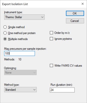
- Open the dialog using File / Export / Isolation List. Set Instrument type Thermo Stellar, select Multiple methods, Max precursors per sample injection to 100, Method type Standard. Note that the max value of 100 is approximate. A smaller number could be required for more narrow peaks or shorter gradients. Press Okay.
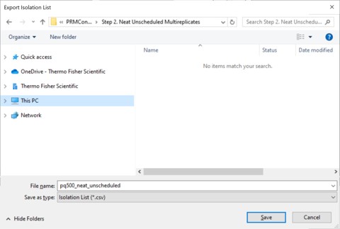
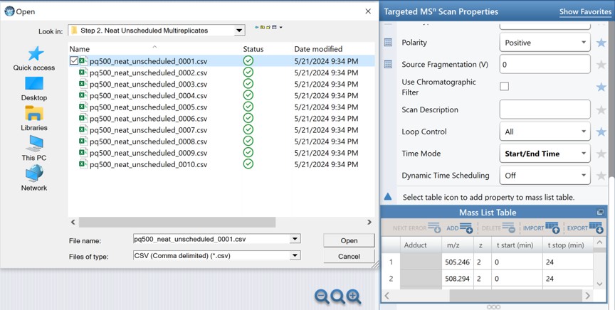
- A Save-As dialog will open. Use the name pq500_neat_unscheduled in the folder Step 2. Neat Unscheduled Multireplicates. In a moment, 10 .csv files with the suffix _0001 to _0010 will appear in the folder. An important aspect of the iRT workflow is that Skyline included the PRTC compounds in each of the 10 files. This allows Skyline to calculate the relative positions of the rest of the peaks, which will eventually be added to our iRT library.
- Open the Stellar method editor and open the file Step 2. Neat Unscheduled Multireplicates/pq500_60spd_neat_multireplicate.meth. In the tMSn experiment in the bottom right you can find the Mass List table and press the Import button to load the first of the created isolation lists, pq500_neat_unscheduled_0001.csv. Use File / Save-As to save the method as pq500_neat_unscheduled_0001.meth. Do this for each of the other 9 isolation lists, creating a total of 10 methods. At this point you would create an Xcalibur sequence with these 10 methods, injecting an appropriate amount of neat standard (ex 10-100 fmol for a 1 ul/min, 24 min assay), and creating 10 raw files. We have performed this experiment for both 60 and 100 SPD methods, and put the resulting .raw files in the folder Step 2. Neat Unscheduled Multireplicates/Raw.
Skyline Method Export
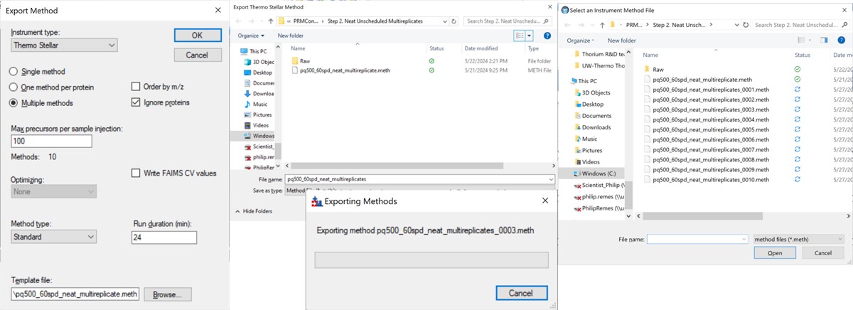
The more convenient way to create the unscheduled replicates is to use the Skyline File/Export/Method functionality. In the Export Method dialog, select Instrument type Thermo Stellar. Select Multiple methods, with Max precursors per sample injection 100. This is a ballpark number that has given enough points per peak for identification purposes for neat standards for a variety of experiment lengths. Click the Browse button and choose the pq500_60spd_neat_multireplicate.meth file in the Step 2. Neat Unscheduled Multireplicates folder. Use a name like pq500_60spd_neat_multireplicates and press Save, and Skyline will present a progress dialog. When it finishes, 10 new methods will be created with suffix _0001 through _0010, as shown below.
Loading Unscheduled PRM Data
- Take the .sky file that we have created, Step 1. Setup Skyline Documents/pq500_60spd_neat_multireplicate.sky and use File / Save As to save a copy with the name Step 2. Neat Unscheduled Multireplicates/pq500_60spd_neat_multireplicate_results.sky. If you want to work along with the 100 SPD method as well, you can save another version of the file with the corresponding name.
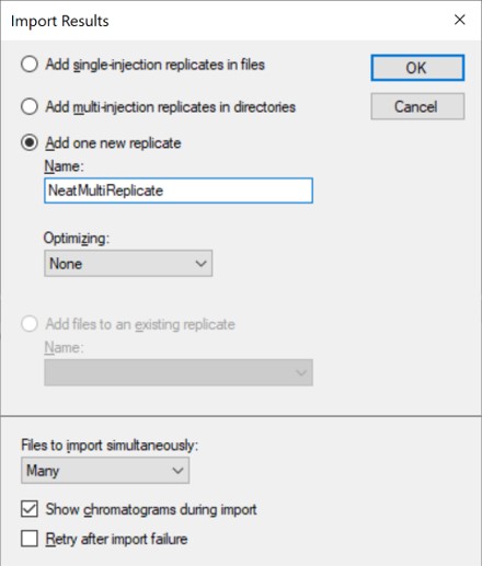
- Use File / Import / Results and select Add one new replicate. Give it the name NeatMultiReplicate. Press Okay, and then select all the raw files in the folder Step 2. Neat Unscheduled Multireplicates\Raw\NeatUnscheduled60SPD and press Open. Skyline will load the results. When they are finished loading, Save the Skyline document. Do the same for the 100 SPD .raw files in their .sky file.
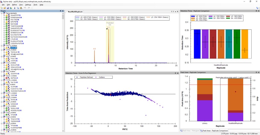
- Now we will inspect the results to see if any peaks have been chosen incorrectly. Use File / Save As to save the Skyline document as Step 2. Neat Unscheduled Multireplicates/pq500_60spd_neat_multireplicate_results_refined.sky (and one for the 100 SPD file).
- Use View / Retention Times / Regression / Score to Run. Right click the plot and select Plot / Residuals. Right click the plot and make sure that Calculator is set to the calculator that we created, PRTC.
- Right click on the plot and select Set Threshold and enter 0.99. If the plot does not update to have some of the blue dots turn pink, then right click the plot and select Plot / Correlation, and then switch back to Plot / Residuals.
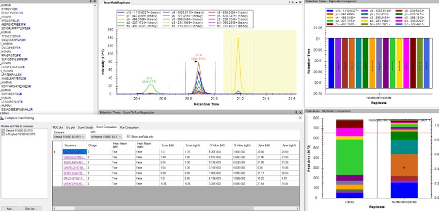
- Use View / Peak Areas / Replicates Comparison and setup the Skyline document something like in the figure below.
Reviewing the Unscheduled PRM Results
Using Score-to-Run RT Outliers
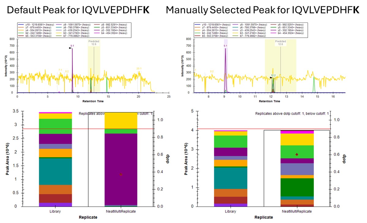
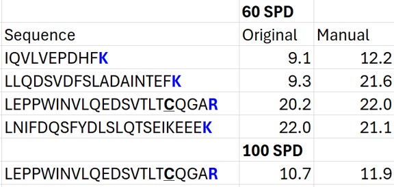
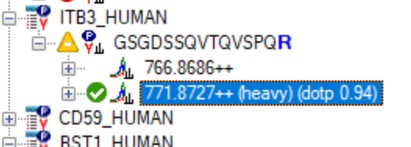
- The Residual Score-to-Run plot is very useful for this step to flag any potential missed peaks. Here we want to click on any of the pink "outlier" dots and inspect them. For example the IQVLVEPDHFK was picked at 9.1 minutes, but the peak in the predicted window at 12.6 has a better library dot product match. Also based on the 100 SPD data, we think that the LLQDSVDFSLADAINTEFK is probably the low intensity peak at 21.6 minutes and not the larger peak at 9.3 minutes that is far away from the predicted RT.
Using Dot Products
-
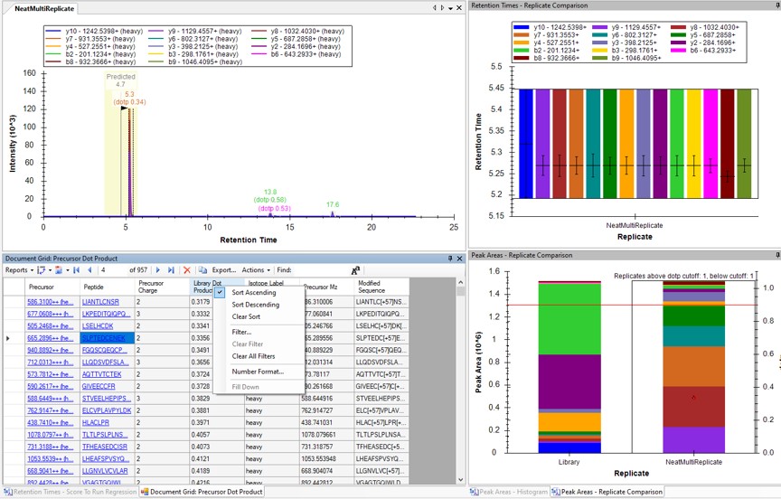
Another way to find picked peak issues like this is to view a Document grid report that has the dot product scores. Use View / Document Grid (or Alt + 3) to bring up the Document grid, and dock it in the same window as the Retention Time Score-to-Run.
- If you ever can't dock a window where you want it, dock the window in some place that Skyline lets you, and then you will be able to dock it where you originally wanted.
-
Click the Precursor Report, then Customize Report to bring up a dialog menu. Erase columns from the right hand side and then click the binoculars and type 'Dot', and press Find Next until you find Library Dot Product. Select this column to add it to the right hand side, and then press okay.
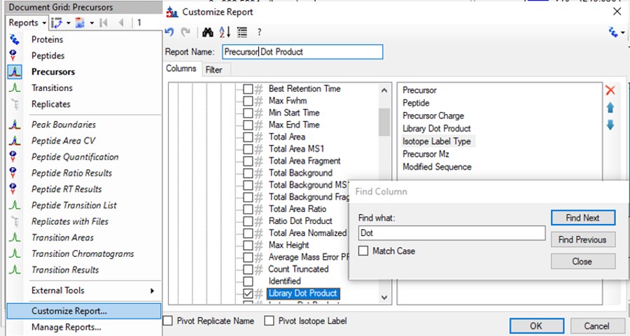
- Now right click on the Library Dot Product column and select Sort Ascending. You can click through on the worse dot product scores to inspect them. Even the ones with poor dot product scores are actually pretty ambiguously belonging to a single precursor at the correct retention time.
Using Peak Picking Models
A final way that can be useful for inspecting this kind of result is to compare the results from the two Skyline peak picking models available at this time. Although in the present case there is not much use for this technique, we'll demonstrate it now.
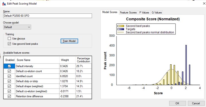
- Select Refine / Reintegrate. In the Peak scoring model dropdown box, select Add. In the dialog that shows up, keep mProphet as the model, and select Training / Use second best peaks. Using decoys is the method used when you have DIA data and have added Decoy peptides to the document. For targeted methods, the second best peak for the peptide serves as the null distribution for training the peak model. Click Train Model. In the feature scores there are several scores that are not available because there are no light peptides in the document. Scroll down the see the enabled features. Several features are red because they decreased the classification accuracy. Unselect those features and press Train Model again, and click Okay to exit the Edit Peak Scoring Model dialog.
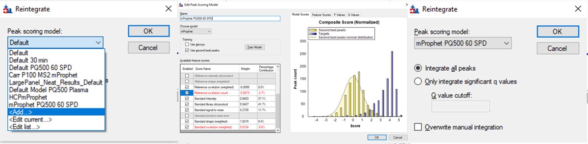
- In the Reintegrate dialog, Add another peak scoring model. This time select the Default model and press Train Model. Then press Okay, and press Okay again in the Reintegrate dialog. This should give us the original peaks selected when the data were imported.
- Go to Refine / Compare Peak Scoring. Use the Add button to add the two peak models that we just made. Go to the Score Comparison tab, select the Default model for the Compare dropdown and the mProphet model for the "with" dropdown. Click the Show conficts only button. Of the 8 conflictin peaks, the greatest ambiguity is probably the first one, LLGNVLVCVLAR. Here there is a very nice peptide peak at 20.9 minutes, but the one at 20.5 although it is further from the predicted RT, has a better dot product. We selected the 20.9 peak, but potentially this is misassigned. We made the same assignment in the 100 SPD method.
Summary of Changes made to Default Skyline Peak Picking
The figure below summarizes the manual changes we made to the Skyline default peak picking. Note that at the time that we first did the study, Skyline could connect to the Prosit server for library generation. By the time this tutorial was written, Skyline was using something called Koina to do the in silico predictions. While the Prosit models are in theory supported, there was an issue with using them. Therefore there could be some small differences. Note that the most conservative approach would be to search the unscheduled PRM data against a PQ500 .fasta file with static R and C heavy modifications, and only select those peptides that passed some threshold FDR value.
Saving a New, Empirical iRT Calculator
- Now we will update the iRT library so that future experiments can benefit from this curated peak picking. Use Settings / Peptide Settings / Prediction, and click the calculator button to Edit Current. In the dialog that opens, click Add in the bottom right corner and add results.., and an Add iRT Peptides dialog announces that 804 peptide iRT values will be replaced. Click Okay. Click Yes when asked if the iRT Standard values should be recalibrated. Now in the iRT database line, use the name pq500_60spd.irtdb, and give it a new name, PQ500+PRTC 60 SPD, press Okay to exit.
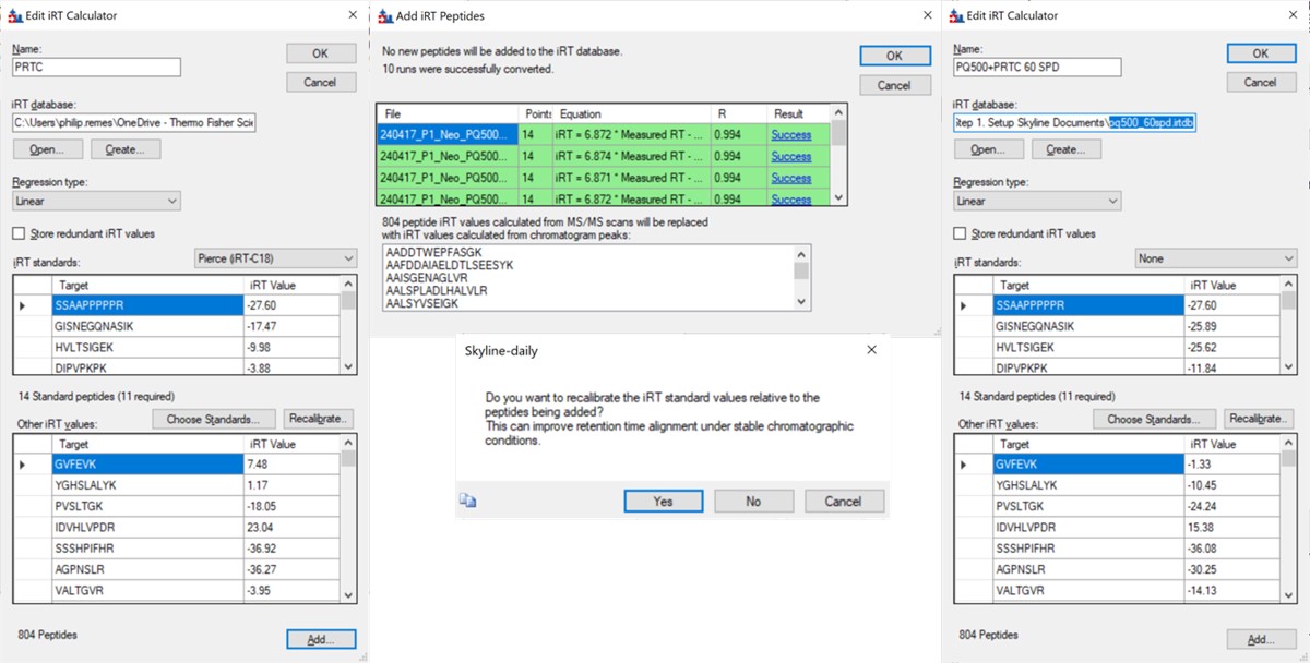
- We've created a new iRT calculator, but have to set it as the active one. Click the calculator icon and Edit List. Press the Add button and then click the dropdown menu, and the new calculator will be there, select that one. Set the Time window to 2 minutes, then press Okay. Select the PQ500+PRTC 60 SPD calculator in the Peptide Settings / Prediction dialog and press Okay to exit to main Skyline window.
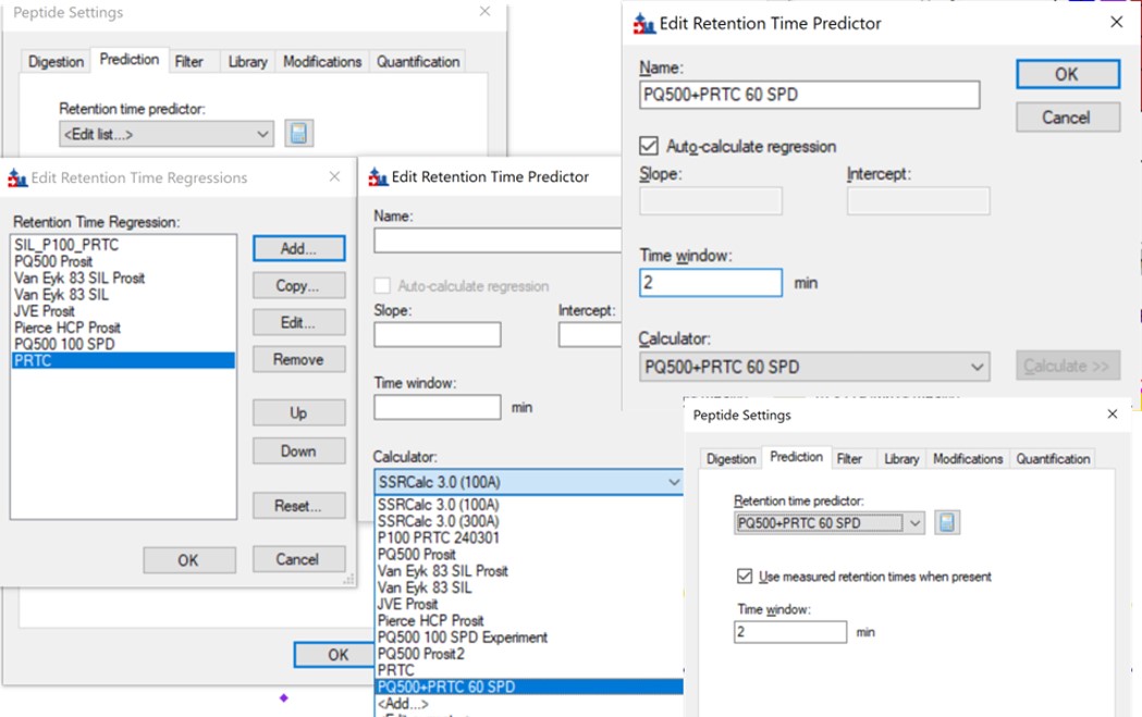
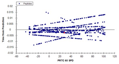
- In the score-to-run plot, right click, select Calculator, and choose the PQ500+PRTC 60 SPD. The plot will update to show an interesting pattern where the errors are all very close to zero. We have now created a new calculator that will make it easier for Skyline to pick peaks next time. We did the exact same set of iRT steps for the 100 SPD Skyline file, because using the new 60 SPD calculator for the 100 SPD does not work perfectly. In the 100 SPD we think that probably the LEPPWINVLQEDSVTLTCQGAR is the peak at 11.9 minutes and not the one at 10.7 minutes.
Filtering Transitions with PRM Conductor
This was a neat sample, but we can filter out the transitions that we don't need at this point, with the understanding that when we spike into plasma we may have to refine the transitions even further.
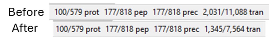
- Select Tools / Thermo / PRM Conductor. The tool opens up. We used the settings in the figure below, where importantly you set Min Good Trans to 5, press Enter, and also select the Keep All Precs box. Press the Send to Skyline button on the bottom left. Save the Skyline document and close the PRM Conductor.
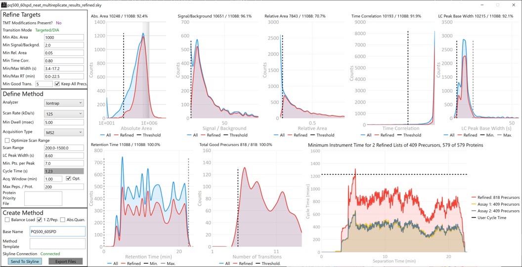
- The number of transitions displayed in the bottom right hand of Skyline will have updated. With the settings we used, the number of transitions dropped from 11,088 to 7,564.
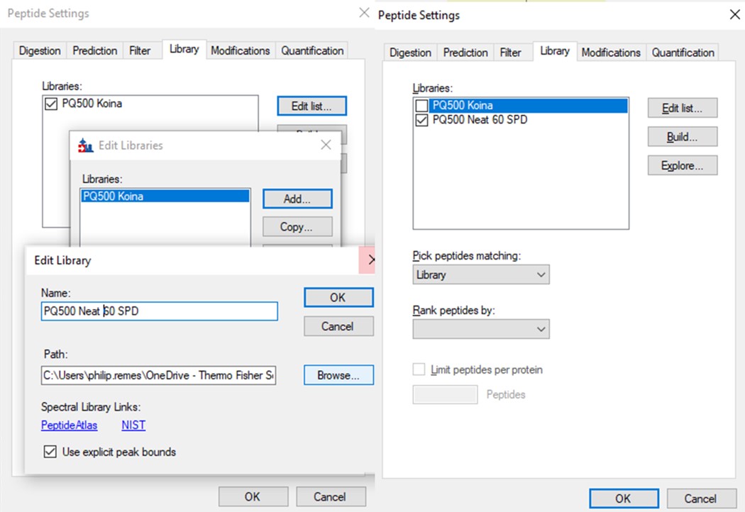
- Use File / Export / Spectral Library and save as Step 2. Neat Unscheduled Multireplicates/PQ500_Neat_60SPD_Refined. Use Settings / Peptide Settings / Library and select Edit List, then Add, and Browse for the file you just saved. Give the library the name PQ500 Neat 60 SPD. Press Okay, and in the Library tab, deselect the PQ500 Koina library and select the new library. Press Okay and save the Skyline document. Make a spectral library in the same way for the 100 SPD document. Close the PRM Conductor instances. We've reached the end of the second step, and are ready to acquire data in plasma.
Plasma Wide Window Scheduled
Scheduled PRM for Heavy PQ500 in Plasma with Wide Acquisition Windows
In this step we will create a wide-window PRM method to verify the RT locations of the PQ500 heavy peptides in plasma. Sometimes it can be the case that the RT’s of peptides will be much different when spiked into matrix compared to when analyzed neat. This is expected and likely due to the binding properties of the chromatography stationary phase, which depend on the concentration of analytes in the liquid phase in an equilibrium sometimes referred to as an isotherm. At the end of this section we will have a candidate final method that includes both heavy and light peptides, and that also includes Adaptive RT real-time chromatogram alignment.
Creating Wide Window Methods that Include Adaptive RT Acquisitions
-
Use File / Save As on our files from the last step, pq500_60spd_neat_multireplicate_results_refined.sky and pq500_100spd_neat_multireplicate_results_refined.sky and save in the folder Step 3. Plasma Heavy-Only Wide Window as pq500_60spd_plasma_multireplicate_results.sky and pq500_100spd_neat_multireplicate_results_refined.sky.
-
Use Tools / Thermo / PRM Conductor.
-
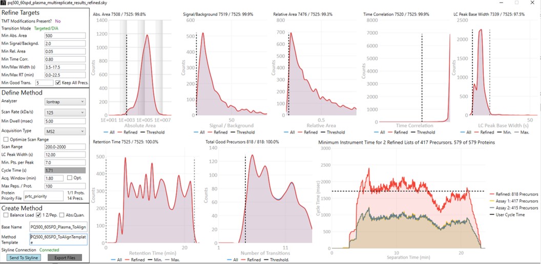
Update the settings as in the figure below. After changing any number value, be sure to press the Enter key on the keyboard. The prtc_priority.prot file is selected by double clicking the Protein Priority File text box. This is just a text file with the line “Pierce standards”, the protein name that Skyline gave to the iRT standards. The peptides from any proteins listed in this file (with Skyline's protein names, not accession numbers) are included in the assay, whether or not their transitions meet the requirements. If the Balance Load checkbox is not selected and there are multiple assays to export, each assay will contain the prioritized proteins, and Skyline will be able to use the iRT calculator for more robust peak picking.
-
Note that with the 1.8 minute acquisition window, the right-most plot in PRM Conductor tells us that the 818 precursors in the assay require up to almost 2500 milliseconds to be acquired, and as we have the Balance load box unchecked, they will be split into 2 assays. If Balance Load was checked, then we would create a single assay, for only the precursors that can be acquired in less than the Cycle Time.
-
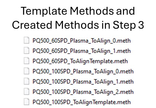
Enter a suitable Base Name like PQ500_60SPD_Plasma_ToAlign. This reflects the fact that we are including acquisitions to perform Adaptive RT, but we are not actually adjusting our scheduling windows in real time. Our neat standards were not suitable for performing aligning in the complex plasma matrix background.
-
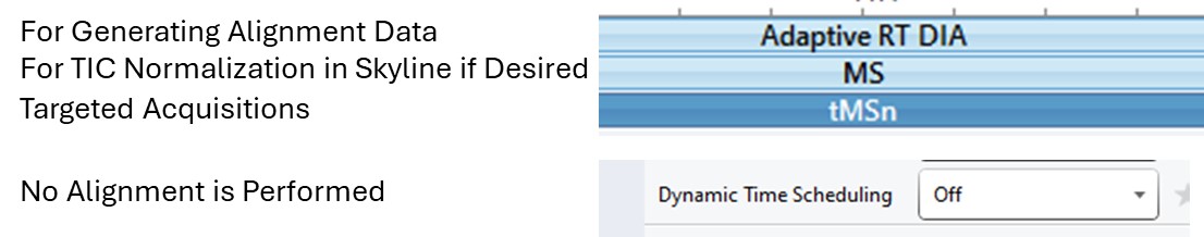
Double click the Method Template field and select the Step 3. Plasma Heavy-Only Wide Window/PQ500_60SPD_ToAlignTemplate.meth file. This file is standard targeted method for Stellar, with 3 experiments. The first is the Adaptive RT DIA experiment, which is being used to gather data for real-time alignment in future targeted methods. The second is a MS1 experiment, which isn't strictly needed, but enables the TIC Normalization feature in Skyline to be used, and can be helpful for diagnostic purposes. Removing it would save on computer disk space. The tMSn experiment can be simply the default tMSn experiment, where we ensure that Dynamic Time Scheduling is Off. If it were on, then PRM Conductor would try to embed alignment spectra from the current data set into the method. Here we leave it off.
-
Press the Export Button. PRM Conductor will open a progress bar and do some work to export a .sky file, and two .meth files with the names PQ500_60SPD_Plasma_ToAlign_0.sky and PQ500_60SPD_Plasma_ToAlign_1.sky. The new .sky file has our new transition list imported and sets the Acquisition mode to PRM. This can be useful especially when discovery data is acquired in a DIA mode, however in this case we want to still compare our neat PQ500 data with the spiked plasma data we’ll be collecting, so we’ll continue using our file pq500_60spd_plasma_multireplicate_results.sky.
-
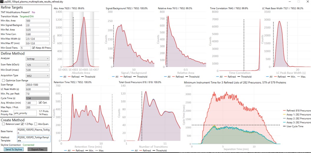
Do the same thing for the 100 SPD method. Here we can create 3 methods if the LC Peak Width is set to 8. Change the Base Name and Method Template to the 100 SPD versions and press Export Files.
- The created methods in this step are as in the figure below. We are now ready to acquire data using these methods. We did this by spiking in PQ500 at the Biognosys recommended concentration into 300 ng of digested plasma that we got from Pierce. Pierce will offer this as a product for sale in the near future (this is written mid-2024).
Reviewing the Wide Window, Plasma, Scheduled PRM Results
-
Open Settings / Transition Settings and set the Retention time filtering option to Use only scans within 1 minutes of MS/MS IDs. You want to be careful with this filtering because if the RT shifts were greater than +/- 1 minute, some data could be missing. You can always use one number and then change it, and use Edit/Manage Results, and select the replicate and Reimport, to use a wider or narrower filter. In this case the IDs are coming from the spectral library that we created in the previous step. Alternatively one could use Use only scans with X minutes of predicted RT option. We need some kind of RT filtering of this sort to help Skyline differentiate between the iRT peptide SSAAPPPPPR and the PQ500 peptide FQASVATPR, which have the same exact m/z.
-
We acquired data for PQ500 spiked into 300 ng of plasma and put the resulting .raw files in the folder Step 3. Plasma Heavy-Only Wide Window\Raw. Load the results with File / Import Results / Add one replicate, use a name like PlasmaMultireplicate, and select the .raw files for the appropriate 60 or 100 SPD throughput. Skyline will load these data files as a single replicate.
-
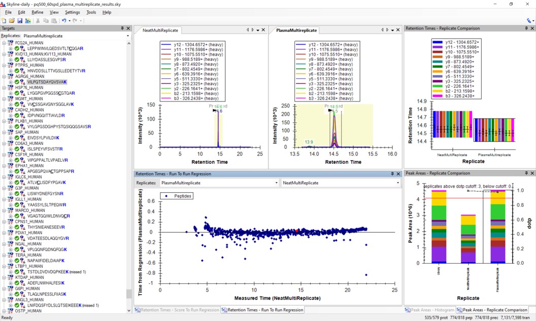
Use View / Arrange Graphs / Row so that we can view the Neat and the Plasma replicates at the same time. Right click a chromatogram plot and use Auto Zoom X Axis / None, so that we are zoomed out as far as we can go.
-
Use View / Retention Times / Regression / Run-to-Run. Your Skyline document should look something like the figure below.
-
Use Save As to save a new version of this file in case we make any changes to the picked peaks. You can use pq500_60spd_plasma_multireplicate_results_refined.sky.
-
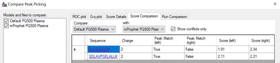
We can do the same steps as above. Make an mProphet and Default Peak picking models with Refine / Reintegrate. Then use Refine / Compare Peak Scoring, select the two new models with the Add button, then select the Score Comparison tab. Select the two models, and click Show conflicts only. We see two descrepancies, and changed the ELLALIQLER peptide from 20.0 to 20.2 minutes, which had a higher dot product and better predicted RT. We kept the default peak for the other peptide.
-
Click on the various outliers and make sure that the peak area plots are showing a good correspondance of the transitions with a high dot product.
-
Use a report with the Library Dot Product sorted from Low-to-High and investigate the worst cases. Even the lowest dot product cases look okay to us.
-
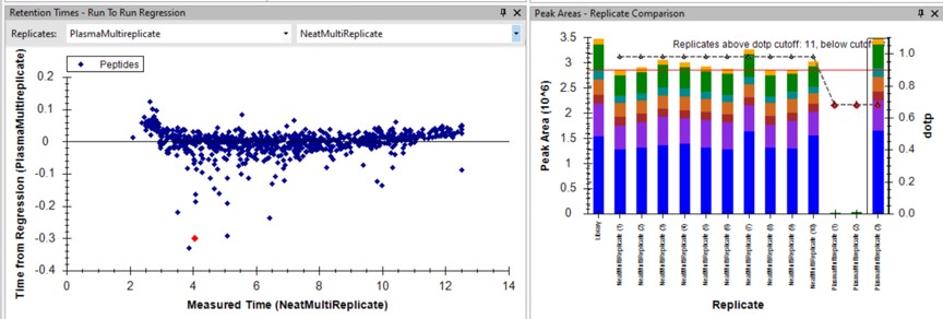
For the 100 SPD data, investigating the Plasma-to-Neat retention times has a similar patterns as for the 60 SPD. There is one case, the FQASVATPR peptide, that has the same exact m/z as the SSAAPPPPPR iRT peptide, which elutes at a similar RT. Reducing the Settings / Transition Settings / RT filtering time to +/- 0.5 minutes can separate these two peptides. We kept all the Skyline picked LC peaks for the 100 SPD document, and saved a new file pq500_100spd_plasma_multireplicate_results_refined.sky.
Creating a Final Method
-
Remove the NeatMultiReplicate using Edit / Manage Results. It's easy to forget to do this. We don’t want PRM Conductor to consider the neat peaks, which are already very clean. Save the Skyline file again.
-
Launch PRM Conductor to clean up interferences and create a final method. Set Min. Good Trans. 5 and check Keep All Precs. Set Min Dwell 5 msec. Set LC Peak Width 11, Min. Pts. Per Peak 7, Acquisition Window 0.6 minutes, and check the Opt. box. This option increases the acquisition windows slightly, especially at the start of the experiment, without going over the user's Cycle Time. Select the prtc_priority.prot file, which in in this case just makes sure that those peptides can't get filtered. Check the Balance Load, 1 Z/prec., and Abs. Quan boxes. This last option instructs the Export command to include light targets for each of the heavy targets. Set a Base Name PQ500_60SPD_Align, and select the PQ500_60SPD_AlignTemplate.meth.
-
This template method is the same as the ToAlign version, only the Dynamic Time Scheduling is set to Adaptive RT. Now when PRM Conductor exports a method, it will compress the qualifying alignment acquisitions in the data and embed them into the created method.
-
We have a small issue here in that there more refined targets (red trace) than we can target. We have to trick PRM Conductor here and set the LC Peak Width to 20 so that all targets are exported, then in the created file change the LC Peak width back to 11 and points per peak to 7. In the future we'll allow the user to just export an "invalid" method.
-
Press Export Files to create the new instrument method.
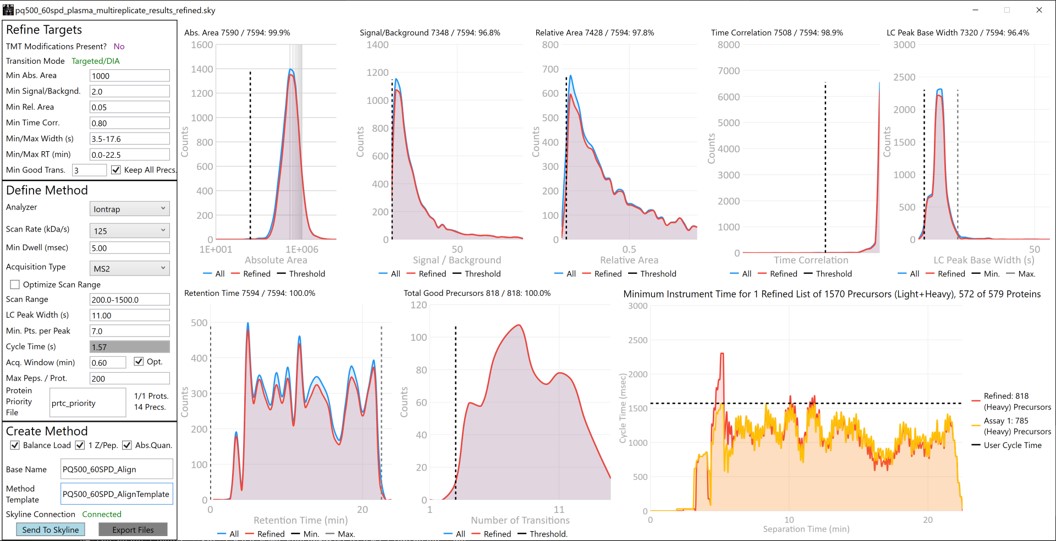
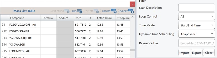
- Open the PQ500_60SPD_Align.meth file, change the LC Peak width from 20 to 11, and the Points per Peak to 7. Note that the Adaptive RT Reference file has a file name that starts with Embedded, and the Mass List table has entries with heavy peptides having names ending in [+10] or [+8] followed by the corresponding light peptides.
-
Use the Send to Skyline to filter the remaining few poor transitions from these targets, and save the Skyline document state. Export a spectral library like we did before, giving it a name like PQ500_60SPD_Plasma. Configure this library in Settings / Peptide Settings / Library. This is the end of step 3.
-
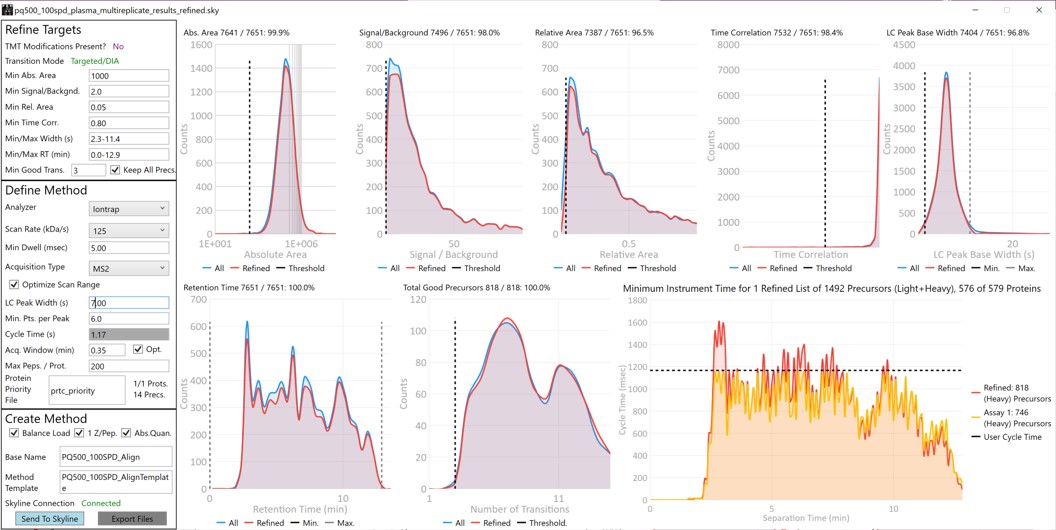
For the 100 SPD case, from the pq500_100spd_plasma_multireplicate_results_refined.sky file, Launch PRM Conductor. Check the Optimize Scan Range box. This will produce targets with customized scan ranges for each target, significantly increasing the acquisition speed, at the cost of some injection time and sensitivity. Set an appropriate Base Name and select the PQ500_100SPD_AlignTemplate.meth for the Method Template. Use the same trick as for the 60 SPD, setting the LC peak width to 20 seconds and Export the method. Then open the method that is created and change the LC peak width back to 7 with 6 points per peak.
-
Press the Send to Skyline button. Export the spectral library and configure it in the Peptide Settings / Library tab. Save the pq500_100spd_plasma_multireplicate_results_refined.sky.
- We now have candidate final methods created for 60 SPD and 100 SPD, respectively PQ500_60SPD_Align.meth and PQ500_100SPD_Align.meth. We are ready to move to the next step and validate the assay.
Plasma Narrow Windows Scheduled
Scheduled PRM for Light-Heavy PQ500 in Plasma with Narrow Acquisition Windows
Analysis of the Heavy Peptides
In step 3 we created two candidate final methods for the 60 and 100 SPD assays. Take the file pq500_60spd_plasma_multireplicate_results_refined.sky and pq500_1000spd_plasma_multireplicate_results_refined.sky, and resave them in the folder Step 4. Plasma Light-Heavy Narrow Window, with names like pq500_60spd_plasma_final_replicates.sky and _pq500_100spd_plasma_final_replicates.sky. In this step we’ll analyze the results of the light/heavy methods created in Step 3. Of particular interest will be the histogram of coefficient of variance values for the peak areas.
-
Use File / Import Results / Add single-injection replicates in files and press Okay. Select the 10 files in Step 4. Plasma Light-Heavy Narrow Window\Raw\60SPDReplicates and press Open. Remove the common prefix and press Okay to load the results. Remove the PlasmaMultiReplicate with Edit / Manage Results and Save the document.
-
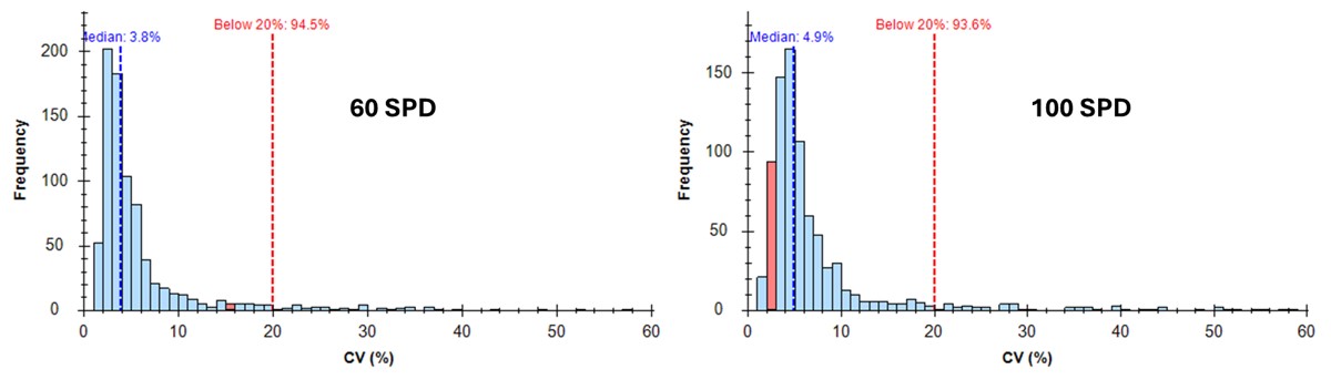
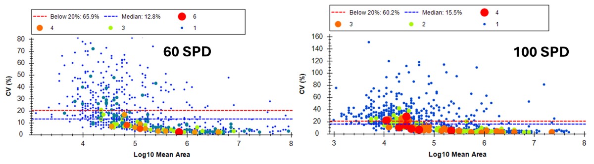
Select View / Peak Areas / CV Histogram. The CV histograms have ~94% of the targets with CV < 20%, with medians of 3.8 and 4.9%, which are excellent.
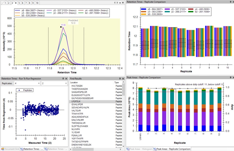
You can click on the histogram, which will open a Find Results window with some of the peptides that are close in CV to the value that was pressed. Double clicking any peptide sequence in the Find Results table will make that peptide active, whereupon one can check the peak shape, peak area, and retention time variations for the 8 replicates. Many/most peptides have results like LFGPDLK below.
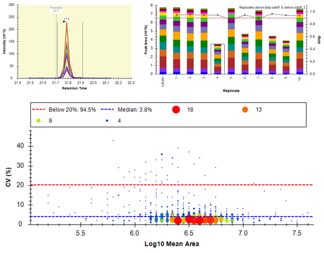
- Another interesting plot is the 2D CV Histogram, found under the View / Peak Areas menu. Here we see that there are 45 targets with CV > 20%. Clicking on the dots makes the peptide in question active. An example peptide SLADELALVDVLEDK is shown below, that has > 20% CV. It has a very skinny peak shape, eluting during the column wash portion of the run. Our analyses show that peptides very early and late in the assays have a high probability of have poor CV. One way to filter these peptides out is based on their narrow peak shape. PRM Conductor can set a minimum LC peak width bounds to do this.
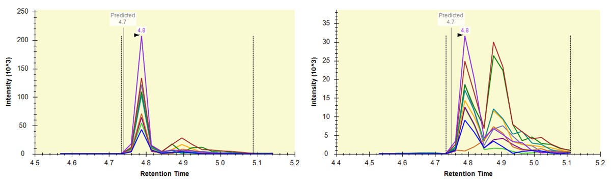
- Some peptides have bad CV's because they have interference an interference that varies from one replicate to another, like ANHEEVLAAGK below.
- One could simply filter all the peptides with a CV greater than a threshold from the document, using Refine / Advanced / Consistency, and set 20% in the CV cutoff box. Or one could try using MS3 acquisition in PRM Conductor, to save those peptides with poor CV's.
Analysis of Both Light and Heavy Peptides
-
Now we will add in the light precursors, that were measured but currently are not in the Skyline document. Save the document and then Save again with the names pq500_60spd_plasma_final_lightheavy_replicates.sky and pq500_100spd_plasma_final_lightheavy_replicates.sky.
-
Use Refine / Advanced, and select the Add box. The Remove label type combo box title changes to Add label type. Select light and press Okay to close the Refine dialog. Each peptide will now have its light precursor added. Use Edit / Manage Results, select all the replicates and press the Reimport button.
- Use View / Peak Areas / 2D CV Histogram, and set Normalized to Heavy. The PQ500 standards were designed to look for a set of proteins of interest, not all of which are expressed in normal plasma. For this reason many of the Light / Heavy area ratios are low, and have high coefficient of variance.
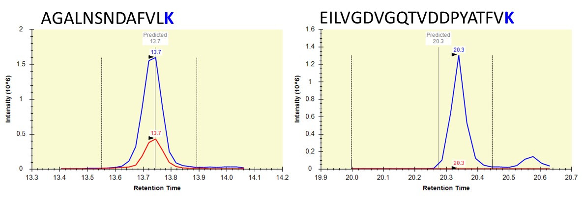
- Some peptides, like AGALNSNDAFVLK have significant endogenous peptide, and therefore have very good CV. Other peptides like EILVGDVGQTVDDPYATFVK have no observable endogenous peptide, and the area ratio therefore has a much higher CV. This general trend is observed in the CV histogram above.
-
This is the end of Step 4. We've demonstrated how to analyze replicate data for absolute quantitation with light and heavy peptides. A next step that some users will want to perform is a dilution curve. For absolute quantitation this takes two forms.
- Heavy Dilution: Constant endogenous (light) peptide amount, varying heavy spike-in concentration
- Light Dilution: Constant heavy spike-in concentration, varying endogenous sample.
-
The Light Dilution is a little easier to perform, because with the Settings / Peptide Settings / Modifications / Internal standard type is set to heavy, and thus Skyline uses the integration boundaries of the heavy peptides to integrate the light signals and determine whether the light/heavy ratios are sufficient for quantitation.
-
The Heavy Dilution is difficult, because eventually Skyline can't find the heavy peptide signal, and doesn't keep a constant integration boundary. Sometimes Skyline will jump over to the next biggest LC peak and ruin the dilution curve. We have sometimes used a script to set constant integration boundaries and solve this issue.
-
Calculating LOQs and LODs for large scale assays is still a little difficult, and we have used python scripts to do this. Skyline is also working on making improvements, and there will be updates in the future. We are submitting a paper soon that will have links to these scripts, for the intrepid that might be interested in exploring them.
Label Free - E. Coli
E. coli Assay Development Overview
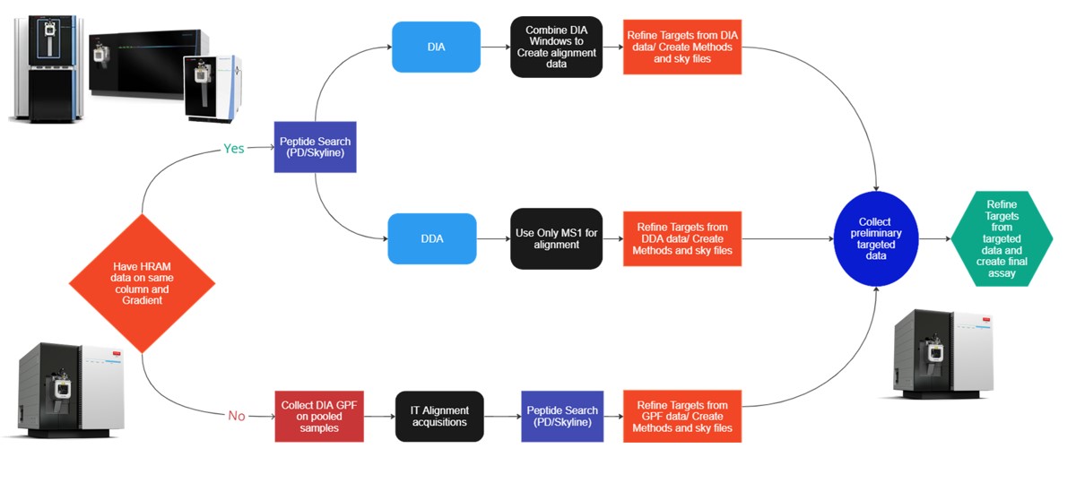
This tutorial will show you how to create a label-free targeted assay from discovery results. As shown in the figure below, there are two main routes to creating this kind of assay, to main difference being whether the discovery data comes from a high resolution accurate mass instrument like Astral, Exploris, or a Tribrid, or whether the discovery data comes from a Stellar. Once we have the discovery results in Skyline, the steps are largely the same. In this tutorial we'll look at an assay created from Stellar MS gas phase fractionation results.
Collect Gas Phase Fractionation Data on Pooled Samples
Overview of the Library Methods
Our recommended technique for creating targeted assays starts with acquiring a set of narrow isolation window DIA data on a pooled or characteristic sample, creating what the MacCoss lab has termed a “chromatogram library”. This technique allows for a deep characterization of the detectable peptides in the sample, and the resulting data can be used to create a Skyline transition list of high quality targets. As outlined in in the figure below, generation of the library typically involves several (~6) LC injections, where each injection is focused on the analysis of a small region of precursor mass-to-charge. This technique has also been called “gas-phase fractionation” (GPF) to contrast with the traditional technique of off-line fraction collection and analysis. The GPF experiment should be performed with the same LC gradient as the final targeted assay, which allows us to use the library data for real-time retention time alignment during later tMS2 experiments.
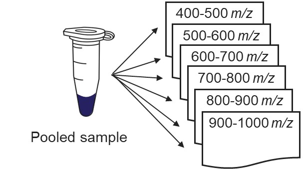
Assuming that a pooled sample is available for analysis, the first step is to create a template instrument method file (.meth). Open the Instrument Setup program from Xcalibur, or the Standalone Method Editor (no LC drivers) if using a Workstation installation.
C:\Program Files\Thermo Scientific\Instruments\TNG\Thorium\1.0\System\Programs\TNGMethodEditor.exe
Use the method editor to open the file at Step 1. DIA GPF/60SPD_DIA_1Th_GPF.meth. This method includes 3 experiments:
- An Adaptive DIA experiment for retention time alignment that has a wide isolation window and ultrafast scan rate. We use Window Optimization Off so that later these windows will not be imported into Skyline, which can be accomplished because both the analytical DIA experiment (experiment #3) and later targeted methods will not use integer precursor m/z values, and Skyline will use a 0.0001 Th tolerance.
- An MS experiment, used for diagnostic purposes. Some DIA processing algorithms may also use the MS data for peptide searching, but currently nominal mass MS data don’t appear to be useful for DIA. Note that MS data can be used for data normalization in Skyline, even when MS data are not being imported.
- An analytical DIA experiment for peptide searching that use a narrow (~1 Th) isolation window. Window Optimization is set to “On” so that isolation window edges are in “forbidden” m/z zones and we don’t have to use any window overlap.
Assuming that the user has configured their LC driver with the Instrument Configuration tool, the LC driver options would appear as a tab in the pane on the left-hand side of the method, where the user has to design the length and type of gradient program to be used. Of course, the choice of gradient length is of great importance as it determines the number of compounds that can be analyzed and the experimental throughput. A general rule of thumb is that Stellar can analyze on the order of 5000 peptides in an hour gradient, where this number depends on how the peptide retention times are distributed and other factors and settings that will be explored later in the tutorial. The user will need to make sure that the MS part of the experiment has the same Method and Experiment Durations as the LC gradient.
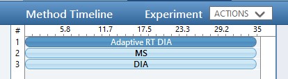
While we are making methods, we should create a tMS2 method template with the same LC parameters as the library method file. One can start with Step 1. DIA GPF/60SPD_tMS2_Template.meth. This method has the same first two experiments as the GPF template, and the 3rd experiment been replaced with a tMSn experiment. Our software tool will later fill in the targeted table information in a new version of this file, as well as update the LC peak width and cycle time parameters and embed the reference data for the Adaptive RT.
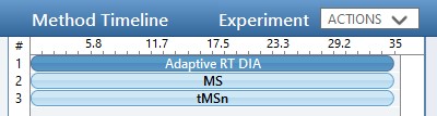
One thing to note about the targeted template is that the Dynamic Time Scheduling is set to Adaptive RT. When we save the method, a message tells us that the file is invalid because no reference file has been specified. This is okay, because PRM Conductor will fill in this information for us later.
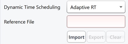
Creating the GPF Methods
Once the GPF method template file is created and saved, the user should select that file with the GPF Creator tool. The tool will create a set of new methods based on this template, one for each precursor mass-to-charge region. The number of method files to be created depends on the settings in the user interface. The default precursor range for the tool is 400 to 1000 Th, as most tryptic peptides have a mass-to-charge ratio in this range. We recommend, for Stellar, to use an isolation width of 1 Th, which allows the DIA data to be searched even with traditional peptide search tools like SEQUEST and allows for a good determination of which transitions will be interference free in the tMS2 experiment. However some users have used 2 Th windows, in order to user slower scan rates and/or more injection time per scan without having to acquire 2x as many GP fractions. If the experiment Maximum Injection Time Mode is set to Auto, then the maximum injection time is the largest value that does not slow down acquisition, which depends on the Scan Rate. For this simple tool, we assume a scan range of 200-1500 Th. The largest amount of injection time and the slowest acquisition rate is afforded by the 33 kDa/s scan rate, and the smallest amount of injection time and the fastest scan rate is afforded by the 200 kDa/s scan rate.
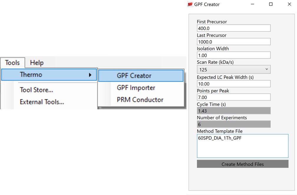
For most applications, we prefer to use 67 or 125 kDa/s and set the Maximum Injection Time Mode to Dynamic as in the figure below, which lets the maximum injection time scale with the time available in the cycle.
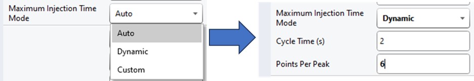
If the Cycle Time is set to 2 seconds and the cycles take less than 2 seconds, then the remaining time in the cycle is distributed to the acquisitions inversely proportionally to the intensity of the precursors, ex. less intense precursors get more injection time. In this figure, the left panel shows a hypothetical situation at the start of a cycle. We calculate the minimum amount of time that each of the acquisitions needs, and sum this to get the blue, vertical, dashed line. The remaining time in the cycle is the white, vertical, dotted line. Each acquisition is colored, with the most intense precursors colored white, based on previous data. In the right panel, the amount of time the acquisitions actually take is displayed, where the less intense precursors were given more injection time.
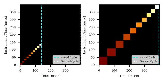
The expected peak width in GPF Creator is the LC peak width at the base in seconds. This value can be determined by checking a few peaks in a quality control (QC) experiment, for example an injection of the Pierce Retention Time Calibration standard. The LC peak width combined with the desired number of sampling points across the peak width, the isolation width, and the Scan Rate determines the number of LC injections needed to create the library.
Once the parameters are set, the user selects the Create Method Files button, which will create the instrument method files needed for the library. The user can create a sequence in Xcalibur and run these methods along with any blanks and QC’s that they want. We have collected data for a mix of 200 ng/ul E. coli with 200 ng/ul HeLa, and placed the resulting raw files in Step 1. DIA GPF\Raw.
Search Library against Organism Database
The next step is to search the data to find candidate peptide targets. Ion trap DIA data with 1 Th isolation windows can be searched for peptides using Proteome Discoverer and the SEQUEST or CHIMERYS search engines. We have included example templates for Proteome Discoverer with this tutorial. SEQUEST in Proteome Discoverer was built to handle data dependent acquisition experiments, and so a few parameters are set to unexpected values. The Precursor Mass Tolerance is set to 0.75 Da, which means that each spectrum is queried against the peptides in a window that is +/- 0.75 * charge_state. For the spectrum selector node, we set Unrecognized Charge Replacements to 2; 3, so that each spectrum is searched as both charge state 2 and 3, because Stellar DIA acquisitions are marked with Charge 0, which is Unrecognized for PD. This practice, plus the wide precursor mass tolerance, means that each spectrum in the chromatogram library takes a long time to search; on the order of an hour for a 30 minute gradient method using a standard instrument PC, ex 6 hours to search a GPF experiment. CHIMERYS searching is often much faster for this kind of experiment.
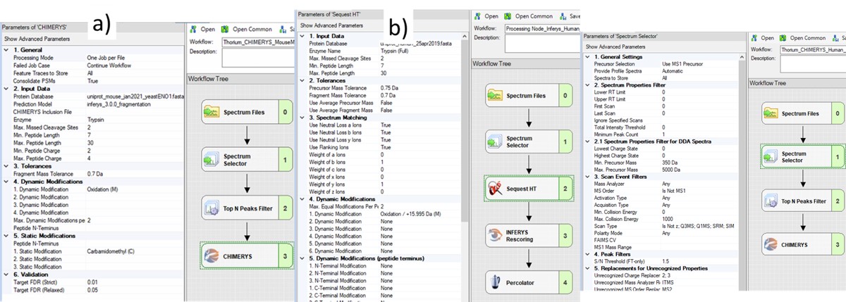
Also, in the spectrum selector node we set the Scan Type to “Is Not Z” (only Full), so that the large isolation width Adaptive RT acquisitions are filtered, which have a Z in the scan header.
A nice, new feature in the Proteome Discoverer 3.1 SP1 is the addition of the Consolidate PSMs option in the Chimerys 1. General section. Setting this parameter to True tells Chimerys to keep on the best PSM per peptide/charge precursor. This consolidation has the effect of speeding up the Consensus workflow significantly, as well as reducing output file size and the amount of time needed for Skyline to import the results.
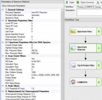
To process the files in Proteome Discoverer, one can first create a study (a), set the study name and directory, and the processing and consensus workflows (b). The workflows can also be set or modified once the study has been created. When the study has been created, one uses Add Files to choose the library raw files, and drags them to the Files for Analysis region, and then presses the Run button to start the analysis (c)
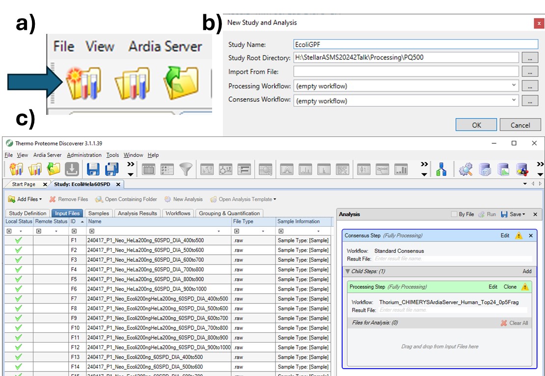
Manual Import Search Results into Skyline
After Proteome Discoverer finishes processing the data, a file is produced with the .pdResult extension, and another one with the .pdResultDetails extension. Both files must be in the same folder for Skyline to import the search results and to start refining a First-Draft targeted method. We will first show you how to import the results manually, and then we will present a simple tool to perform the import with the settings that we recommend for ion trap analysis. To import the PD results manually, create a new Skyline document, and save it as ImportedGPFResults\gpf_results_manual.sky. Open Settings \ Peptide Settings, and set the parameters as in the figure below. The main points are to ensure that no Library is selected, and the Modifications do not specify any isotope modifications. Skyline will check for Structural modifications in the imported search results and ask you about any that are not already specified. Press Okay on the Peptide Settings dialog box.
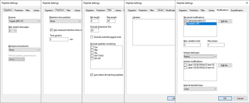
Open the Settings \ Transition Settings and use settings like below. Set Precursor charges to 2, 3, 4, Ion charges to 1,2, and Ion types to y,b. Don’t specify ‘p’ in Ion types, because PRM Conductor currently takes this as a sign that DDA is being used and loses some functionality. Set Product ion selection from ion 2 to last ion. For Ion match tolerance use 0.5 m/z, with a maximum of 15 product ions, filtered from product ions. Set the Min m/z to 200, and Max m/z to 1500 (whatever was used for acquiring the GPF data), with Method match tolerance of 0.0001. Set MS1 filtering to None, and MS/MS filtering to Acquisition method DIA, Product mass analyzer QIT with Resolution 0.5. For the Isolation scheme, if a suitable scheme is not yet created, select Add. Here we set 0.35 for the Retention time filtering, but a wider window may be more acceptable for longer gradients.
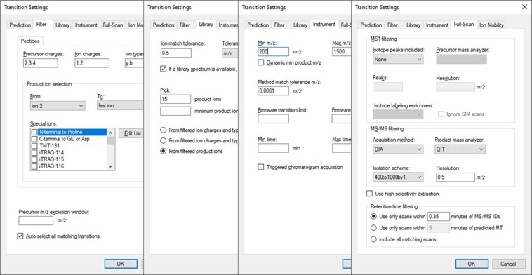
As below, once Add is selected for Isolation Scheme, give it a suitably descriptive name, then press Calculate. Set the Start and End m/z to the limits and isolation width used in the GPF experiment, and click the Optimize window placement button, assuming you used that option in the GPF experiment. Press Ok twice to close the Isolation Scheme Editor, and once more to close the Transition Settings.
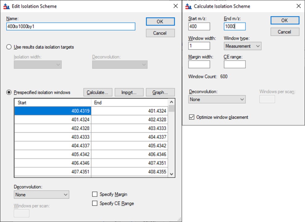
Save your Skyline document at this point, and select File / Import / Peptide Search. Use the Add Files button to navigate to and select the Step 1. DIA GPF/Processing/240417_P1_Neo_Ecoli200ngHeLa200ng_60SPD_DIA.pdResult file.
As in Figure below, select Score Threshold 0.01, Workflow DIA and press Next. Skyline will build a .blib file from the .pdResult, which will take several minutes. If you get an error during this step, ensure that the .pdResultDetails file is also present in the same folder as the .pdResult file, for PD >= 3.1, and ensure that you are using an updated version of Skyline (preferably the Daily version). When this step finishes, Skyline presents a .raw file chooser dialog, select Browse and select the files in Raw / GPF. Press Next, then you can remove or not remove portions of the file names to shorten them, and press Okay. The next Add Modifications tab should be empty if the Peptide Settings / Modifications were already specified, so press Next again. In the Configure Transition Settings, Skyline will have overwritten several of your Transition settings, so remove the ‘p’ from Ion types, and set Ion match tolerance to 0.5, and Max product ions 15, Min 3 and press Next. In the Configure Full Scan Settings, set the MS1 Isotope Peaks to None, and press Next. In the Import FASTA tool, Browse and select the .fasta file in the Processing folder. You can set the Decoy generation to None, especially if you used PSM Consolidation to reduce to a single PSM per peptide, then press Finish. Skyline will start associating peptides to proteins now, displaying a progress bar, and eventually shows an Associate Proteins tool. Here the most strict setting would be to create protein groups and remove any peptides that are not unique to a protein, but alternatively one might choose to Assign to the first gene, for example. Press Okay, and Skyline will import the results from the .raw file, which may take a few minutes. Note that one could have skipped the results importing and pressed cancel at any time after the library was created. The library would be available to browse with View / Spectral Libraries, and the peptides could be added to the document with Add All. Occasionally this process can be used if there were any errors or issues with modifications. Additionally one could use this strategy to load the .raw files as a single multi-injection replicate, the way that the GPF Importer will do, which makes viewing the results much more convenient as we’ll see below. When the results are finished loading, save the gpf_results_manual.sky file.
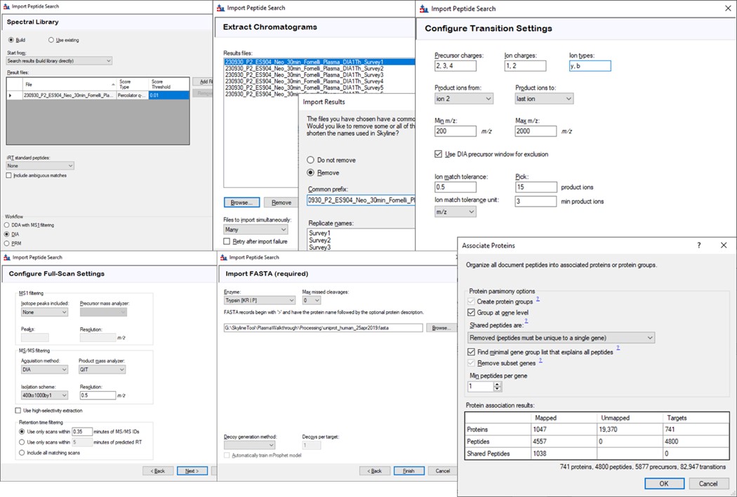
Click on the second gene labeled greA to expand it. Notice that with the 600to700 file selected, only two peptides are visible. With the scheme we have used, each .raw file was loaded on its own, instead of as part of a whole. To see the difference, use Edit / Manage Results (or Ctrl+R) to open the Manage Results tool, press Remove All and Okay. Now use File / Import / Results. When asked if you want to use decoys say No. In the Import Results tool, select Add one new replicate and use the name GPFMultiReplicate, and press Okay. Choose the six .raw files in the Raw / GPF folder again, and they will be immediately imported if you had finished the importing with the Wizard. The greA gene that is expanded now will have all its peptides completely filled in, like below. Save the gpf_results_manual.sky document.
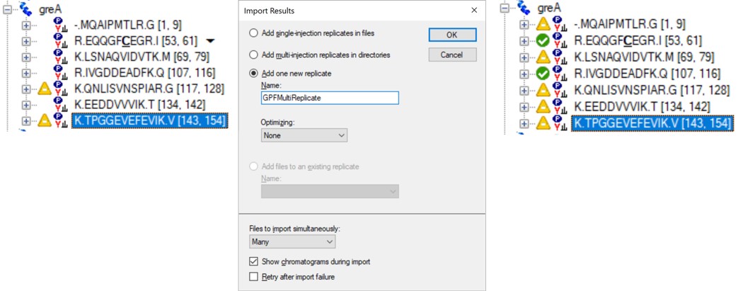
GPF Import Search Results into Skyline
We’ll now look at how the GPF Importer does the same thing as above, but with fewer steps. To use the GPF Importer tool use Tools / Thermo / GPF Importer. Double click the Peptide Search and FASTA file boxes to select the .pdResult file and FASTA file respectively. In the Output file Path, Copy/Paste in the output directory you want, and type an appropriate name for the new Skyline file. Double-click the Raw File pane and select the associated GPF .raw files and press the Import to Skyline button. The log window shows the progress of the import, which takes several minutes. When it finishes, the result will be the same as in the figure below when the multi-injection replicate was imported.
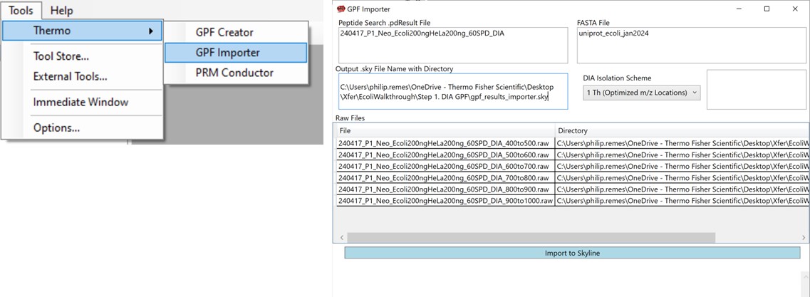
This is the end of the first step. We have Skyline files with peptide search results in them. In the next steps we'll refine the results on our way to making a final assay.
Validation with Subset Replicates
- Refining the Search Results
Refining the Search Results
Use PRM Conductor Skyline plugin to refine the transitions and precursors
Launching PRM Conductor
Once the results are imported into Skyline, the next step is to create a First-Draft version of the targeted assay using the PRM Conductor Skyline plugin. If you followed the steps in the tutorial, the Step 1. DIA GPF / gpf_results_importer.sky file should have opened after the import was finished, or you have the gpf_results_manual.sky version made. From one of these files, launch the PRM Conductor program (a), and Skyline’s bottom bar will report the progress of creating a Skyline custom report file that gets loaded by PRM Conductor (Figure b). Note that PRM Conductor depends on .raw files for some analysis, so it will look in obvious locations for the data files referenced in the Skyline file. If the raw files were not found, it will ask you to find the missing files. Once you double-click and use the file chooser to select them, the dialog will show a green “True” and you can continue. Even if the Skyline file used .mzml or another raw file format, just place the associated .raw files in a nearby folder and you can use the PRM Conductor.
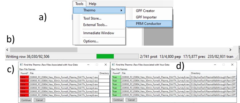
Once loaded, the user interface in the figure below will be shown. There are 3 main parts to the user interface: a set of parameters on the left, a set of transition metric plots on the top right, and a set of precursor metric plots on the bottom right. We start with the Refine Targets parameters and the associated plots. Each of the text boxes has a corresponding graph on the right. The current value in the text box is a threshold value, and is displayed with the graph as a dashed, vertical line. The title of the plot reports how many of the transitions were filtered based on the current threshold. The blue distribution in the plot is for all the transitions in the report, while the red one is after all filters have been applied. Changing the parameter in the text box and pressing Enter will update the calculations in the plots on the right.
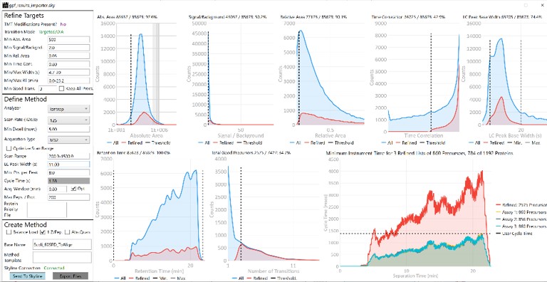
Refine Targets Section
The first plot on the top is Absolute Area distribution. These are the Area values determined by Skyline for each transition. Note that these values are analyzer dependent, so a threshold used for Orbitrap discovery data may not be suitable for the Ion trap discovery data. The second plot is the Signal/Background distribution. These are the values of Area and Background as determined by Skyline for each transition. A traditional threshold for S/B is 3, however the user may wish to adjust to a different value. Highlighting the blue distribution and left-clicking will bring up a new window that gives the user an idea of what a particular S/B looks like in the Skyline transition data. For example, the figure below is a view of the plot after clicking the Signal / Background plot around 4. In the top left, all the transitions are in a grid, sorted by Signal / Background. On the bottom left is a grid showing all the transitions for the peptide corresponding to the selected transition on the top left grid. The graph on the right shows all the transitions for this peptide. The selected transition is highlighted in dashed lines. All transitions that currently meet the thresholds are colored blue, while the other transitions are colored grey. The red transition is the median transition trace.
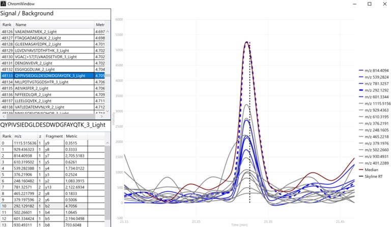
The third plot on the top is the Relative Area distributions, that is, the area normalized to the largest transition for each precursor. The fourth plot is for the time correlation of each transition to the median transition for each precursor. The fifth plot on the top is for width of the transitions at the base, where a general rule is that outliers from this distribution may be poor quantitative markers, either because they are too narrow to characterize with the same acquisition period as wider peaks or are wide and potentially not reproducible. On the bottom row, the first plot is the retention time distributions. Precursors that are at the very beginning and very end may have the highest variability and could potentially be filtered out. The final transition filtering parameter is the Min Good Transitions text box. Many researchers prefer to set this value in the range of 3-5, to increase the confidence that a set of transitions is a unique signature for a peptide of interest. However, you could also click the Keep All Precs checkbox if you wanted to keep all the precursors, along with their best Min Good Transitions, which would potentially include some “bad” transitions. This is useful for cases with heavy standards where you don’t want to remove any of them. This is used in the Absolute Quantitation - PQ500 walkthrough.
Define Method Section
The next set of parameters on the left, in the Define Method box, control the acquisition parameters to be used in the targeted method. These parameters affect the speed of acquisition and the number of targets that can be scheduled in an analysis. The first parameter in the Define Method box is Analyzer. In this tutorial we are focused on Ion Trap analysis, but it is possible to make assays for other Analyzers. Selecting an Analyzer makes a specific set of parameters visible, which can change the characteristics of the analysis.
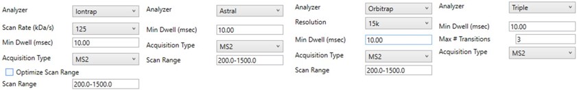
When any of these parameters are updated, the Scheduling graph on the bottom right will update. This graph shows the distribution of retention times for all Refined precursors in the red trace and the user’s chosen Cycle Time with the horizontal, dashed, black line. As we will see later, the user can choose to create a single assay that schedules as many precursors as will fit beneath that Cycle Time or may choose to create as many assays as necessary to acquire data for all refined precursors. The figure below shows views of the Scheduling graph in the single assay or “Load Balancing” mode, which we will talk more about below.
For peptide analysis, there is not much practical utility for the additional resolution afforded by the 66 kDa/s or 33 kDa/s over the “unit mass resolution” of the 125 kDa/s scan rate. Because for targeted methods we typically use the Dynamic Maximum Injection Time Mode in the instrument method file, the instrument allocates any additional time in the cycle to the targets according to their intensity. Therefore, the slower scan rates historically were useful mostly to guarantee a minimum amount of injection time per target, above the ~13 ms afforded by 125 kDa/s with the 200-1500 Th Scan Range, which can be useful for low concentration samples. With PRM Conductor, one can also set a minimum injection (or dwell time for QQQ users), which can accomplish the same thing. For peptides, we typically use the fixed 200-1500 Th scan range, because it guarantees this amount of injection time, gives a reasonable acquisition speed (~65 Hz), and the fragment ions in regions above and below this range are not essential to characterize most tryptic peptides.
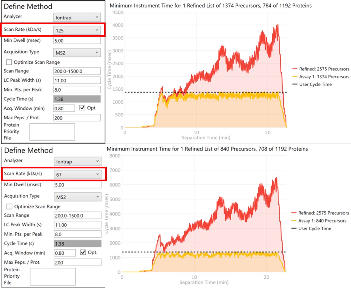
Let’s see what effect the Scan Rate has on the experiment. Changing the Scan Rate updates the estimation of how fast the instrument can acquire data. This is reflected in the Minimum Instrument Time plots, where in the top view, the Scan Rate is set to 125 kDa/s. An assay that would acquire data for all 2575 Refined Precursors would take 4 sec at the peak (at ~21 min), and 1374 precursors are able to be scheduled with the user-defined Cycle Time of 1.38 seconds. When the Scan Rate is set to 66 kDa/s (bottom part of the figure) the 2575 Refined Precursors would take 6.5 seconds of instrument time, and only 840 precursors can be scheduled with a Cycle Time of 1.38 seconds.
The user can change any of the parameters in this pane and visualize the effect on the assay. Of particular importance is the Acquisition Window. Stellar instruments are enabled with a new algorithm for real-time chromatogram alignment called Adaptive RT, which allows the instrument to adjust when targets are acquired to account for elution time drift. We find that an Acquisition Window setting of 0.75-1.00 minute usually results in good data, at least for the gradients we have typically used, in the range of 30 to 60 minutes. As LC peak width decreases for shorter gradients, we have successfully used narrower Acquisition Windows of 0.5 or even 0.3 minutes. Traditional tMS2 experiments, without real-time alignment, can sometimes require Acquisition Windows in the range of 3-5+ minutes. Adjusting this parameter allows to visualize the gain in number of targets afforded by narrower Acquisition Windows. For example, a 1 minute versus a 5 minute Acquisition Window allows to analyze more than 3x more targets (1172 versus 305). An additional feature related to Acquisition Window is the Opt check box. We have observed that the most variable part of many separations is at the beginning, which poses additional challenges for a real-time alignment algorithm because few if any compounds are eluting at the beginning. The Opt checkbox expands the Acquisition Windows somewhat, while still respecting the user’s Cycle Time requirement. The targets that are most improved by this algorithm are the early and late eluting targets; those where expanding their acquisition windows has little effect on the available injection time, but where alignment can be the trickiest.
The last two parameters, which will be explored more below, are the Max Peptides per Protein, which helps to focus the analysis on just the highest quality peptides from each protein, and the Protein Priority File, which allows to create exceptions for particular proteins using their Skyline protein names.
Create First-Draft Targeted methods and Skyline analysis file
Exporting Multiple Methods for All Refined Precursors
Now we will create multiple tMS2 methods for all the precursors that passed the filters and check to see which ones are stable and reproducible quantitative targets. To do this, uncheck the Balance Load button, which changes the Minimum Instrument Time plot so that all the Refined precursors are split into 3 assays, each of which require less acquisition time than the 1.38 second Cycle Time. Enter a base name for the file that will be created, otherwise the name “assay” will be used. Double-click the Method Template box and find the Step 2. Validation with Subsets/60SPD_PQ500PRTC_AlignTemplate.meth file. Then click the Export Files button.
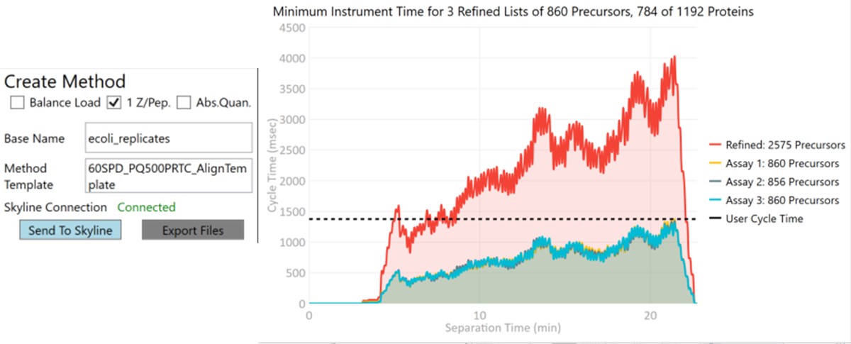
Some processing of the raw files will take place, as denoted by a progress bar, while the data files are aligned in time and a Adaptive RT reference file with the .rtbin extension is created. This processing only happens once, so if PRM Conductor is ever launched again for these raw files it won’t take as long to Export. The processing can take several minutes, depending on how many files are present and how long the gradient was. Method files will be created for each of the 3 assays in the same folder as the tempate method. A Skyline file will be created that is configured for tMS2 analysis with settings appropriate for the selected Analyzer. As a backup for the method and Skyline files, isolation and transition lists lists will be saved that are suitable for importing to the method editor or Skyline. The figure below is a view of the Step 1 folder showing some of the created files, and also the Step 2 folder showing the exported method files.
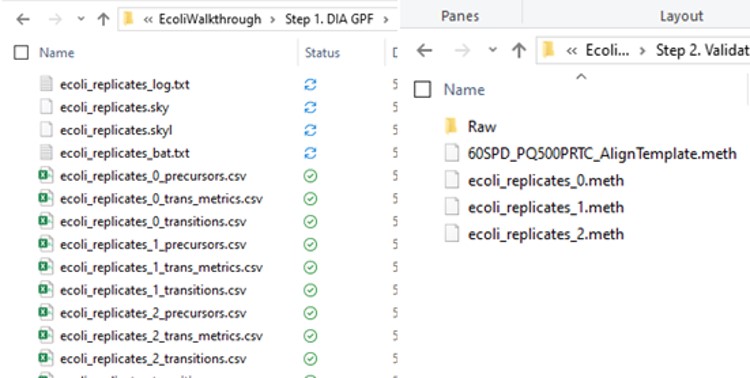
Note that because the 60SPD_PQ500PRTC_AlignTemplate.meth file had an Adaptive RT experiment and the tMSn method had Dynamic Time Scheduling set to Adaptive RT, the methods have embedded a .rtbin file to use for the real-time alignment. Notice too that the user’s Cycle Time and Points Per Peak were included, as well as the relevant precursors with their m/z, z, and scheduled acquisition times.
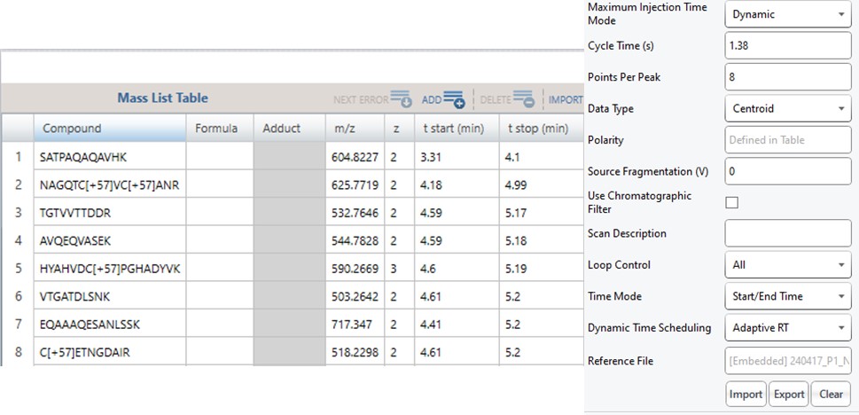
When exporting method files, a feature that can be useful is the Protein Priority File. There are two reasons to use this feature:
- when exporting multiple replicates, the peptides from any proteins on this list will be added to each of the replicates. The purpose of this is to support Skyline’s iRT feature, which requires the same iRT peptides to be present in each replicate. We explore this more in the walkthrough on absolute quantitation.
- When exporting a single replicate (balance load mode), any peptides from proteins on this list are added to the final list, assuming they passed the transition and precursor filters. To use the Protein Priority File feature, just create a text file with the .prot extension, and add any prioritized proteins to it, one per line, using exactly the format that Skyline uses for the Protein Name. For example, one could add sp|P00350|6PGD_ECOLI, as seen in the figure below in the Protein document grid, but not the Gene name displayed in the Skyline tree. When the .prot file is selected, the UI updates to display how many proteins and peptides are being prioritized. For this walkthrough we didn’t use the Protein Priority File feature, however.
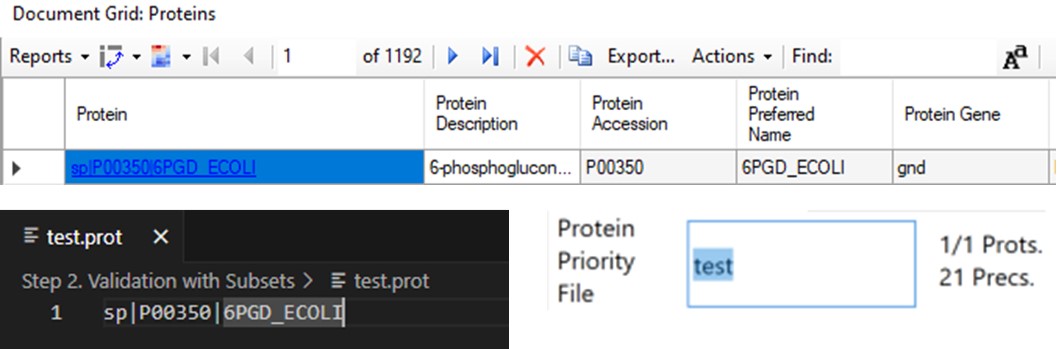
Acquire First-Draft Targeted data on Stellar MS
If the user desired, they could rely on just the results from the library to create a targeted assay. However, because a targeted assay may be used for many samples, we have found it worth the extra effort to further validate the set of precursors for reproducibility by performing several injections with each of the first-draft assays and filtering on a minimum coefficient of variation (CV) on the LC Peak Areas. In some more advanced scenarios where the assay is part of a multi-proteome mixture, one could perform injections for at least two concentrations of the proteome of interest, to ensure that the selected peptides change area with concentration appropriately, and thus belong to that proteome. In this tutorial we will demonstrate filtering performed on the LC peak area CV.
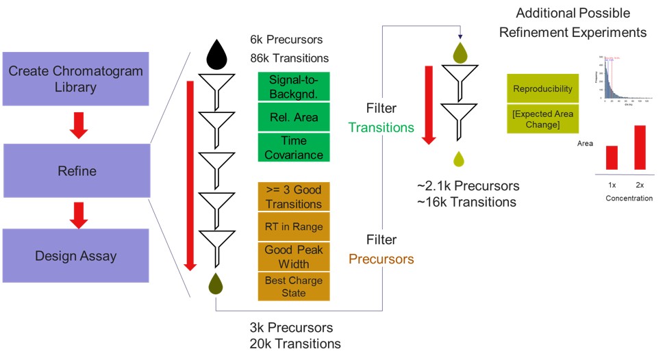
Import First-Draft results to Skyline
We performed 2 injections for the 3 first-draft assays. The program was in a slightly different state at the time, so the data collected don’t perfectly match the Skyline file created in the previous step, but they are very close. Normally we could just use the ecoli_replicates.sky file created in the last step for importing the results, but because of the different program state, we'll instead do a Save As on the Step 1. DIA GPF/gpf_results_importer.sky and save a new file, Step 2. Validation with Subsets/ecoli_subset_replicates.sky.
- Change the Transition Settings / Full Scan / Acquisition method to PRM with QIT analysis, and set the Retention Time filtering to a value that will probably cover the retention time shifts in the coming weeks that this assay will be run, +/- 2 minutes.
- Use Edit / Manage Results and remove the Chrom_Lib_Replicate.
- Use File / Import / Results and select Add multi-injection replicates in directories, and then choose the Step 2. Validation with Subsets\Raw folder in the dialog that pops up. Press Okay and we can also Not remove the common 'Replicate' in the folder names. Loading the data as multi-injection replicates, them nicer to view in Skyline, because each of the multiple raw files involved in a replicate is merged into a single result, and peptides won’t show up as “missing” if the wrong result file is selected.
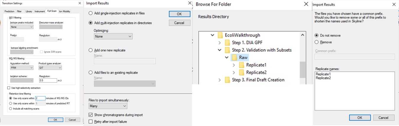
- Now though because we started from the gpf_results_importer.sky that has all the peptides, we should Refine / Remove missing results, and then Refine / Remove empty proteins.
- Arrange the graphs like in the figure below.
- View / Retention Times / Replicate Comparison
- View / Retention Times / Regression / Run-to-Run
- View / Peak Areas / Replicate Comparison
- View / Peak Areas / CV Histogram
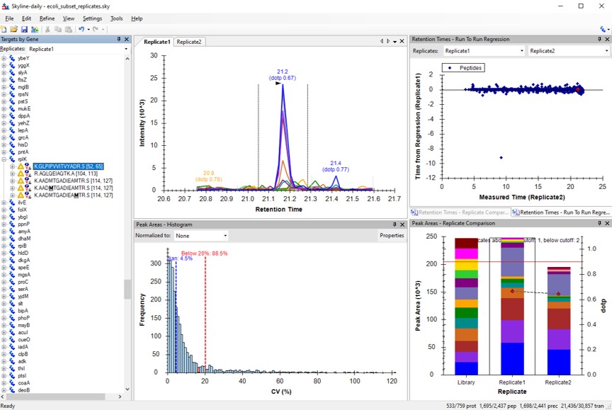
Final-Draft Creation
CV Refinement in Skyline
We have kind of a chicken-and-egg dilema now. As the .sky document currently has all of the up to 15 library transitions for each peptide, should we filter them first, and then filter the precursors by CV, or should we filter by CV and then filter the transitions? Here we opted to do the following to explore all the different options:
- Use Save As and save ecoli_subset_replicates_refined.sky. Sometimes when you save the document, the transitions go back to their original state. So it's better to save the document before you make any big changes.
- This switching of the transitions back to their original state happens if Settings / Transition Settings / Filter / Auto-select all matching transitions is selected. Go there and unselect that option, and press Okay.
- Run Tools / Thermo / PRM Conductor
- Select the Keep All Precs. option, so that we don't filter precursors, and keep a minimum of 3 transitions for each one. If there are only 2 good transitions, the 3rd one will be the next highest scoring, where the score is intensity x time_correlation.
- Press the Send to Skyline Button
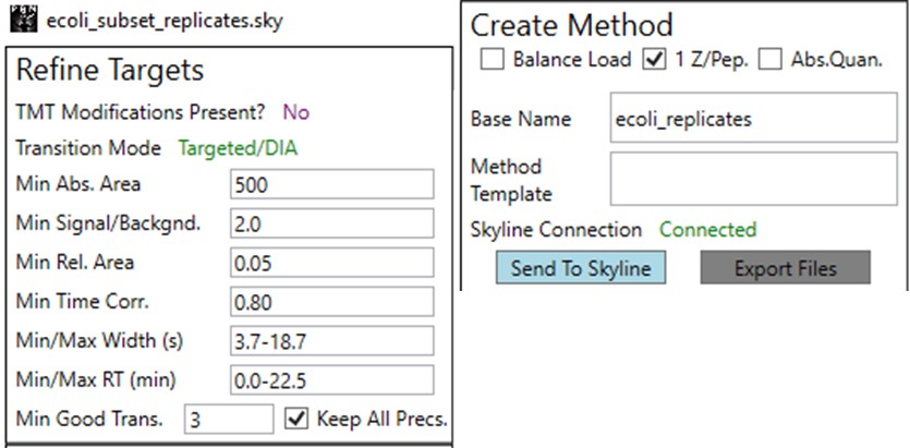
You can use the undo/redo buttons to see the effect that the filtering has had on the transitions. For example, in the figure below is shown the data for the AQLQEWIAQTK peptide before and after filtering.
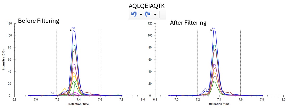
- One can click on the CV histogram, and Skyline opens a Find Results pane, that allows you to click on peptides and explore what the peaks look like at various CVs. You could also use View / Peak Areas / CV 2D Histogram to see a rather typical plot, where the most abundant peptides have the lowest CV's, in general, although bad CVs can be found at almost any intensity. Or good CVs at low intensity, for that matter.
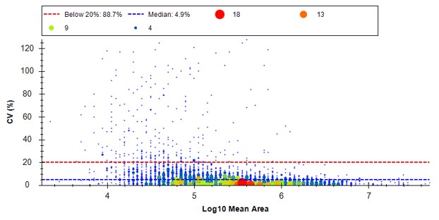
Because we have a MS experiment in our method, the Total Ion Current normalization method is used, which can help normalize out experimental variation like autosampler loading amounts.
- Save the Skyline file as ecoli_subset_replicates_refined_cv.sky.
- Use Refine / Advanced / Consistency and enter 30 in the CV cutoff %. If you were going to use TIC Normalization, then be sure to select that option in the Normalize to: combo box. Press Okay. The CV histograms will update, and the number of proteins, peptides, precursors, and transitions will update in the bottom right hand corner of the Skyline document. You can use the undo/redo to check the effect. Save the Skyline document.
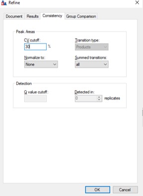
Filtering + Load Balancing
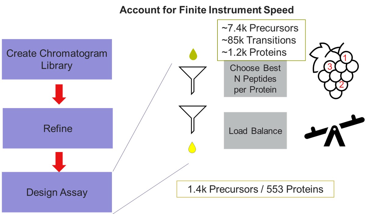
Now we will design the Final Draft assay. Our goal for this section is to ensure that the instrument can acquire quality data all the targets that are of interest. Here the experimenter can make certain concessions, such as, how many peptides per protein would give a usable result? Or am I willing to use 7 points across the peak instead of 10? We send the data to the PRM Conductor tool for analysis again using Tools/Thermo/PRM Conductor and get a View of the program like below. Compared to the earlier figure when PRM Conductor was run on the discovery results, these graphs are much different, because the precursors and transitions picked were already of such high quality. The percentage of transitions retained in the titles of each graph is close to 90% or greater. We set the LC Peak width to an even 11 seconds after hovering our mouse over the LC Peak Base Width graph to see the apex width, and set the Acquisition Window to 0.8 min.
This assay is what we would currently consider "normal", or conservative. There are 1411 precursors in a 24 minute method, which is about 3.5k precursors/hour. Had there been more precursors at earlier retention times, these settings would give about 5k precursors/hour. For fun, we have included HeLa results in the Step 1. DIA GPF\Processing\HeLaResults folder for those that wanted to explore what happens with a massive number of possible precursors.
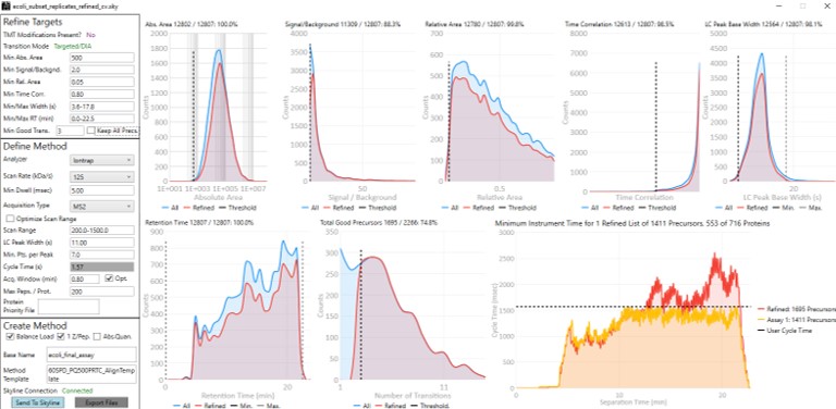
To realize the maximum throughput on Stellar MS, the user can select the Optimize Scan Range button, and could try using 6 points per peak, which is sometimes considered to be the Nyquist frequency for a Gaussian peak. We have successfully used such settings and observed little change in the results. The tradeoff being made with these settings is in the minimum amount of injection time per acquisition.
- The conservative mode guarantees about 13 milliseconds of injection time, because that's the largest injection time that doesn't slow down an HCD acquisition. If you made a method with the Maximum Injection Time mode set to Auto in the Method Editor, this is the injection time you would get. We like to use the Dynamic Maximum Injection Time Mode, where the precursors that have extra time in the their cycle, like the ones at 8 minutes, would get that extra time distributed to them.
- The aggressive mode only guarantees as much injection time as would not slow down the acquisition that has a customized scan range for the transitions that pass the PRM Conductor filters. This could be as little as the value in the Min Dwell Time box, currently set to 5 milliseconds. The rule-of-thumb is that signal-to-noise goes up (and LOQs get better) as the square root of the injection time.
- If you export a method with the Optimize Scan Range, you can see all the various, customized scan rates for each precursor.
- This mode can achieve more than 8000 peptides/hour throughputs. Play with the HeLa results to check this out.
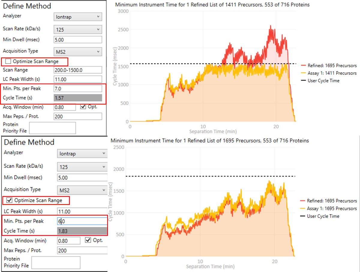
Create Final-Draft Targeted Method and Skyline file
Notice that in above figures, the Balance Load check box is checked, and so the yellow Assay 1 trace in the Minimum Instrument Time plot is flattened up against the user Cycle Time. If the Max. Peps/Prot. value was reduced from 200 to 2, then the assay would contain only 869 precursors precursors, and there would be more space between the top of the Assay 1 trace and the horizontal cycle time line. Peptides are added from each protein in order of their quality from highest to lowest, as long as there is time at that point in the assay, and as long as the protein being considered has less than Max. Peps/Prot. peptides scheduled. It’s possible that an assay with fewer targets would have better quantitative performance, due to the longer available maximum injection times, and that could be of interest to the experimenter. In this example we leave the Max Peps./Prot. value at 200.
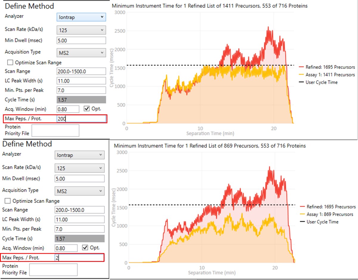
- Click on Export Files to export a method. Once again, some processing takes place as the raw files are analyzed, and finally isolation and precursor lists, as well as method and Skyline files are created. This is the final draft assay, ready to be used for targeted experiments.
- Normally we would use either the created Skyline file to collect our next data sets, or we would Save the current Skyline file with a new name, and press Send to Skyline from PRM Conductor to update it. In this case, because as mentioned above, the subset validation assays were slightly different when the data were collected compared to this walkthrough, we'll use the Skyline file actually used for data collection in the next step.
Analysis of Final Assay Replicates
Final Assay Replicates
Many researchers are not quite done once they have a "final-assay". Typically users want to perform a larger number of replicate injections with this candidate assay. A typical practice for assays that will be used for a large number of samples is to characterize the stability of the peptides and reproducibility of the LC/MS system using a 5x5 experiment. In this experiment, 5 different samples are digested and prepared, and each aliquoted into 5 vials, for 25 total. The vials are stored in the autosampler or a refridgerator at the same temperature, and each day for 5 days in a row, at least 5 replicates are acquired for each of the 5 vials. The inter-day, intra-day, and inter-sample variability can be assessed, and poorly performing peptides can be removed.
Here we will simply load some replicate data acquired with a final assay very similar to the one that we created in Step 2 of the walkthrough.
A Note about Spectral Libraries
An action that we could have included at the end of Step 2 is to create a final spectral library, once all the final peptides are refined and their retention times are known. In the future when replicates are imported, the retention time filtering for MS/MS IDs will be relative to the spectral library you have created, and not from the discovery runs, which can be useful. We can do this from the Step 2. Validation with Subsets\ecoli_subset_replicates_refined_cv.sky file.
- Use File / Export / Spectral Library
- You could use a name like ecoli_final_assay in the dialog that pops up. Note that when we exported a final method in the last step, the script actually created that library, so you don't have to overwrite it.
- To use the new library, you go to Settings / Peptide Settings / Library, and Edit list.
- Move the cursor to the bottom of the list, so the new library will be added there. Press Add.
- Find the location of the library you made, and give it a name.
- Then unselect the previous library, and select the new library.
- Press Okay to exit. Now the new library is being used.
- As it is, we'll use the library that comes with the file Step 3. Final Draft Replicates\ecoli_large_replicates.sky. Open this file.
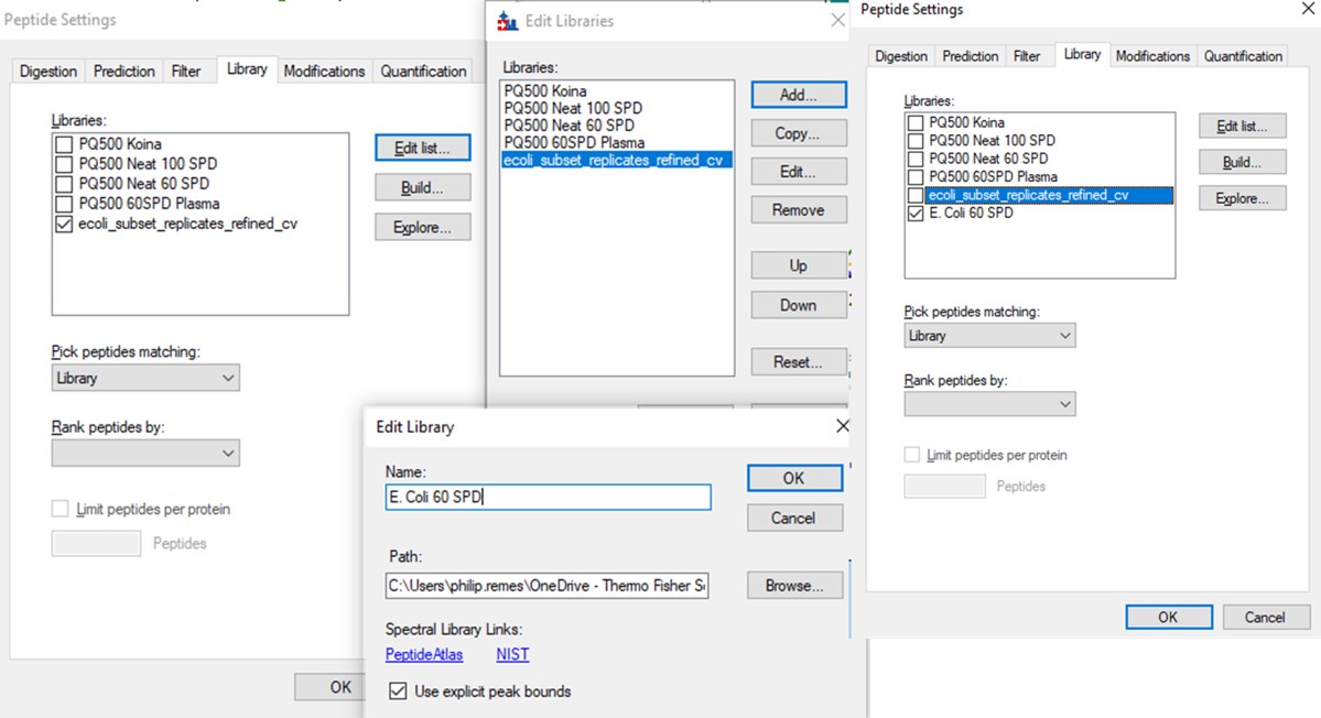
Loading and Analyzing the Results
- Use File / Import / Add single-injection replicates in files, and add the 8 files in Step 3. Final Draft Replicates\Raw.
- After these load, you can arrange the Skyline document as before.
- Save the Skyline file as ecoli_large_replicates_loaded.sky.
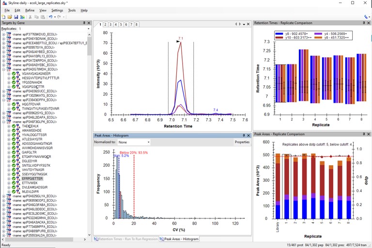
Use View / Retention Times / Regression / Run-to-Run. There are some peaks that are not consistently picked. Click on any of these outliers to see what they look like. Most are some kind of noise. Maybe they were "reproducible noise" in a previous step, or maybe there are interferences that get picked up over time with multiple replicates.
We could filter out the remaining peptides with poor CV's. This actually gets rid of all but a few of the retention time outliers. Additionally we could run PRM Conductor, and set some more stringent filtering settings, like in the figure below. We would unclick the Balance Load box to ensure that no precursors are filtered based on whether they fit in less than the cycle time, and press Send to Skyline.
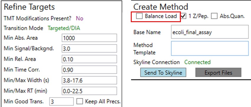
Here we see the effect on the retention time outliers from run to run. Almost all the outliers are gone.
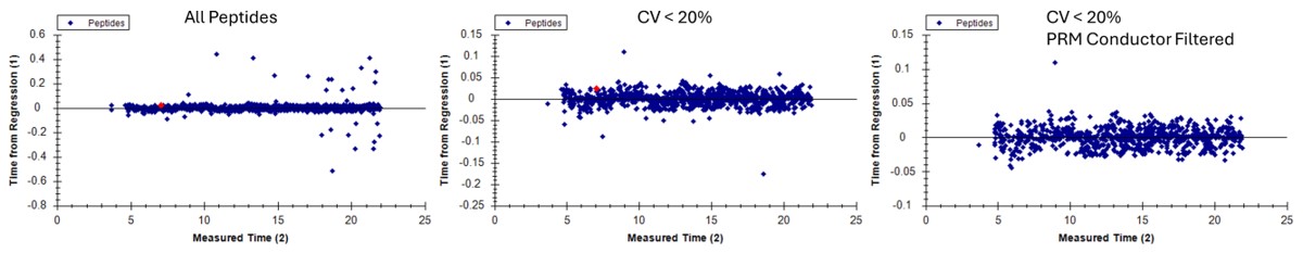
- Make sure that Settings / Transitions Setttings / Filter / Auto-select all matching transitions is not selected, and then Save As ecoli_large_replicates_loaded_refined.sky. This assay is has removed a few precursors, and could be used going forward.
Filtering Retention Time Outliers in Another Way
Let's try another way of filtering the retention time outliers. Go back and open the file Step 2. Validation with Subsets\ecoli_subset_replicates_refined_cv.sky.
- Open Settings / Peptide Settings / Prediction.
- Select Add from the Retention time predictor drop down menu.
- Select Add from the Calculator drop down menu.
- In the iRT standards drop down, select Add.
- In the Calibrate iRT Calculator, press Use Results, and enter a number like 100 in the Add Standard Peptides dialog that comes up, and press Okay.
- Give the Calculator a name like E. Coli PRM Assay and press OKay in the Calibrate iRT Calculator.
- In the Edit iRT Calculator, press Add Results, and then Press okay when asked to add these peptides, and if the standards should be updated.
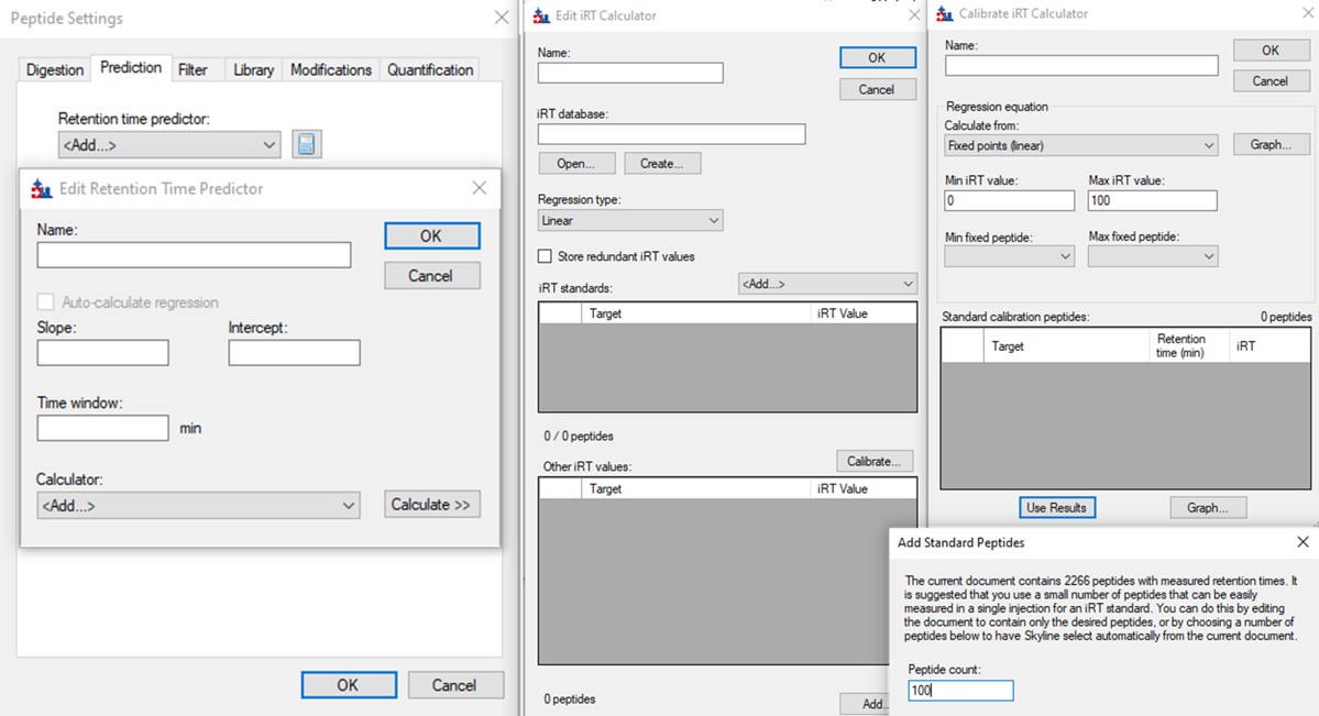
- Press Create on the iRT database button, and select Yes when ased to create a new database file. Save as Step 3. Final Draft Replicates/ecoli_irt_prm.irtdb.
- In the Edit iRT Calculator dialog still, give it a name like E. Coli PRM and press Okay.
- In the Edit Retention Time Predictor, set 2 minutes, and press Okay.
- We are still in the ecoli_subset_replicates_refined_cv.sky file, so we don't need to use the calculator here. Set None in the Retention time predictor, press Cancel, and close this Skyline file.
- Open up our ecoli_large_replicates_loaded.sky file, where we have all the retention time outliers.
- Go to Settings / Peptide Settings / Prediction and the E. Coli PRM name should be there. If it wasn't, for some reason, you could add the calculator we created from the Edit List option. Select the E. Coli PRM calculator.
- We were asked to add some standard peptides, because some of the ones that went into the calculator are not present. You can add them or not add them.
The background of the chromatogram plots is now beige, and there is a faint vertical line that says "Predicted" on the plots, like below.
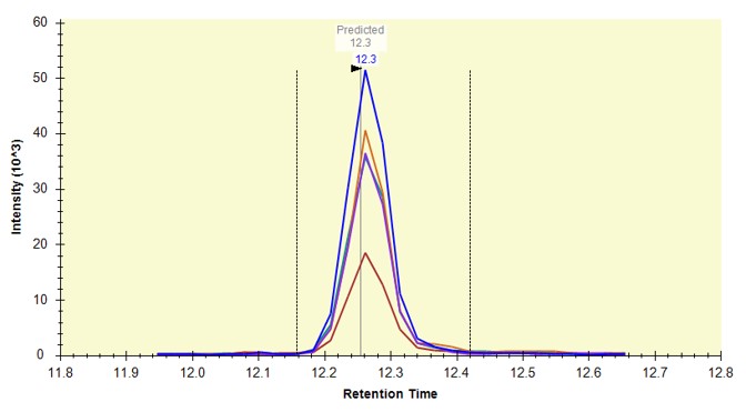
Use View / Retention Times / Regression / Score-to-Run, and on the plot that comes up, right click and in the Calculator menu, select the E. Coli PRM. Make sure that you are in the right-click, Plot / Residuals mode. Some of the dots in the plot are pink just because our document here has some peptides that weren't in the calculator. That's fine for this walkthrough.
- Use Refine / Advanced / Results and set Retention time outliers to 0.999 and press Okay. These peptides that were pink dots are now removed.
- You can do the same thing by right clicking the plot and setting the threshold, and then right clicking again and selecting Remove outliers.
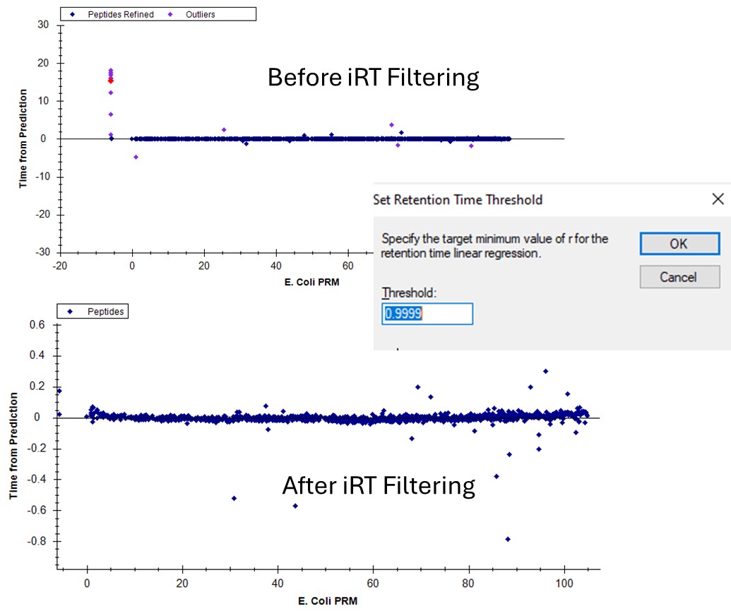
If we go back to the Run-to-Run regression, there are still a few outliers. Apparently we can't yet filter based on the experimental Run-to-Run deviations, but maybe in the future. This iRT filtering maybe wasn't as powerful in this example as just using the CV and PRM Conductor filtering, but it's another tool in our belt.
You've reached the end of this tutorial. Hopefully have a good idea of how to create an assay based on Stellar MS discovery results.
Known Issues
Known Issues
In the following sub-pages, we'll list any issues that we know about, and their workarounds.
Stack Overflow when Exporting Methods
Stack Overflow Error Message - 7/9/2024
Update for Stellar 1.1 software in mid-2025 - this issue was fixed! The following steps are only needed for Stellar 1.0.
Stellar 1.0 Fix
The mechanism used to create methods from a template has failed on occasion with a Stack Overflow message. This can happen with method export from:
- Skyline using File / Export / Method
- GPF Creator when creating sets of DIA methods
- PRM Conductor when exporting an assay to a targeted method
We think that the Thermo method export library loads certain assemblies, and that it is possible that another process loads them first and renders them unusable by our programs. Running our processes as an administrator seems to fix the problem across multiple launches of Skyline.
Solution 1: Running Skyline as an Administrator
Select Tools / Thermo / GPF Creator to launch this program. In Skyline, the immediate window opens that displays the path to GPF Creator.
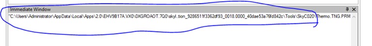
Copy paste this path into a windows explorer path, removing the parenthesis " before the C:\Users. Go up one level past the Tools folder, and sort the files by Type, and the Skyline-Daily.exe will be visible. Close the current instance of Skyline and right click the executable and run as an Administrator.
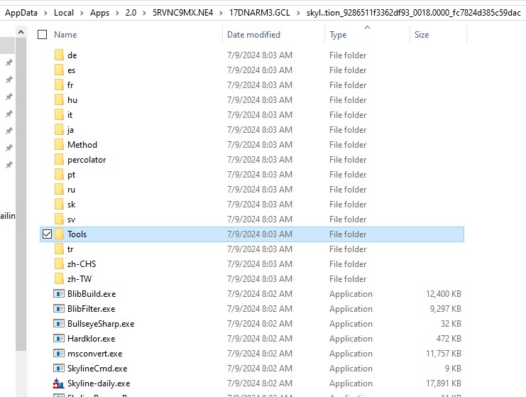
Solution 2: Running GPF Creator as an Administrator
We think that Solution 1 will work, but on a previous instance, before I had realized that Skyline-Daily.exe was in the folder one up from Tools, I fixed the problem by running GPF Creator as an administrator and exporting a method. This allowed methods to be exported from Skyline, GPF Creator, or PRM Conductor across multiple program launches and computer restarts.
- Like for Solution 1, open a windows explorer folder but this time in the folder where GPF Creator is.
- Right-click the Thermo.TNG.PRMBuilder.SurveyCreator and run as an Administrator.
- The GPF Creator application will launch.
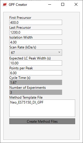
- Select a method that has a DIA experiment in it. We have attached a dia method, but you can also easy build one, but opening method editor, selecting the Hybrid view button, and double-clicking the DIA Scan in the MSn menu on the left.
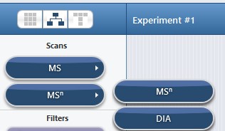
- This will add the DIA experiment to the time line. Save the file, and then in GPF Creator, double click the Method Template file box and select this file, and press the Create Method Files button. This should create the new template methods as normal, and free up the Thermo method export libraries for future calls.
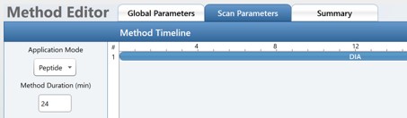
Hypothesis-driven discovery with Multiple Target Monitoring
Hypothesis-driven discovery on Stellar MS
Multiple target monitoring


Experimental design
In this tutorial, we will be dealing with 3 proteome mix consisting of 3 samples:
A: 50 ng Human/45 ng Yeast/ 5 ng E. coli
B: 50 ng Human/ 37.5 ng Yeast/ 12.5 ng E. Coli
C: 50 ng Human/25 ng Yeast/ 25 ng E. coli
D: 50 ng Human/ 12.5 ng Yeast/ 37.5 ng E. coli
E: 50 ng Human/ 5 ng Yeast/ 45 ng E. coli
We are acquiring data with 28-minute gradient to achieve a mix of throughput and coverage.
Tutorial files

Step 1: Pilot experiments with gas phase fractionation
Gas phase fractionation DIA
To start, we will acquire gas phase fractionated DIA data. Here, we will simulate a pilot experiment, where we acquire GPF data on several pooled samples to identify differentially expressed proteins. This tutorial has a brief overview of building a chromatogram library. More detailed information can be found in Label Free- E. coli tutorial.
Building methods
We begin by making a template method with an adaptive RT experiment and DIA experiment. The template method should have:
- LC parameters to be used in the final experiment
- Source settings to be used in the final experiment
- Adaptive RT DIA experiment spanning the full LC gradient
- DIA experiment with appropriate settings (DIA window parameters don’t matter as they will be updated shortly)


The template method is in the Raw Data folder, titled: GPFDIA_28min_1Th.meth.
Open Skyline on a computer with instrument control software installed (you should be able to open .meth files in Method Editor on this computer), ensure that most recent version of PRM Conductor is installed from Tool Store. Open the GPF Creator tool.

Update the settings, select the template method file, and export the template methods.

GPF creator will save GPF DIA methods to the folder that contains the template method. Create an Xcalibur queue and run the GPF DIA data on desired samples.
Searching Stellar GPF data
Search the data in Proteome Discoverer with Chimerys, using Stellar_GPF_Chimerys.pdProcessingWF and the standard consensus workflow.


Note that we changed CE for DIA experiment to 27% in our template method, so we have a max collision energy filter to avoid searching any of the alignment spectra. This will need to be removed if the DIA experiment used the default CE of 30%. Assuming that the adaptive RT experiment used the 200 kDa/s scan rate, the scan headers for its acquisitions will have a 'Z' character in them, corresponding to the legacy Zoom scan rate. Therefore, the Scan Event Filter, Scan Type Is Not z can filter out these adaptive RT acquisitions, and the CE filter is not strictly needed.

Here, I only searched the GPF data for sample C to build the library. I would recommend even with a pilot experiment to search one pooled sample to build the library from. This will simplify assay creation. If the samples are not similar enough, more samples may be searched here.
Filtering search results in Skyline
Importing results

Filtering for quality peptides
Now, we want to go ahead and filter for well-behaved peptides. First, we want to clean up data just a bit.
Go to settings > Transition settings and add a scan filter as shown to ensure that no alignment spectra are imported.

Then go to to Edit > Manage Results and reimport Chrom_Lib_Replicate to ensure there are no more alignment spectra in file.

Now, we can use PRM Conductor to filter for peptides with good peaks. Open the PRM Conductor external tool. You can play around with parameters under Refine targets, this is better explained in other tutorials. I used the following settings:

Ignore the Define Method section and go down to Create method. Uncheck box that says “Balance load”. If you were to export a method from here, PRM Conductor would create enough individual PRM methods to cover all the peptides in library. Here we want to further process the data, so instead of clicking Export Files, click “Send to Skyline”.

This will give you a Skyline document refined for peptides IDed at 1% FDR with “good” chromatographic peaks. This reduced the document from 8637 proteins/ 43341 peptides to 4591 proteins/ 14480 peptides.
Filtering data based on pilot experiment
After refining the GPF data, you may want to further refine the list of peptides based on pilot experiment. There are many ways that one could do this, like generating multiple PRM assays with PRM Conductor and running on samples from different conditions, or doing wider window DIA data. In this case, I had decided to do a pilot experiment on 2 different 3 proteome mixes, so I could filter for quantitative peptides.
Import each GPF replicate by selecting “Add new replicate” and selecting all GPF files:

After this step, you will end up with 3Proteome_28min_GPFDIA_PRMConductorRefined.sky.
Peak picking in pilot experiment
Because we didn’t search these GPF runs in the library, we don’t know if the peak picking is good. So an optional next step is to perform Expert Review analysis with the GPF run we did search as reference. To do this, save the document and then open the Expert Review External tool.
Select “Current” reference file, then check the GPF run(s) that you searched in PD. We will assume that this has correct retention times. Click Start to begin peak picking.

Once peak picking is finished, you will see live view of peak picking metrics. More information on this can be found in Expert Review tutorial. Click Send to sync boundaries to Skyline.

At the end of this, you should end up with something like 3Proteome_28min_GPFDIA_PRMConductorRefined_ER.sky.
Exporting quantitative information from pilot experiment
Now that we have pilot data imported with corrected peaks, we can process the data and apply filters. Here, we will export a quantitation report and filter for peptides that are within factor of 2 of expected fold change between samples A and E. To get quantitative data from Skyline, open Document Grid (View > Live Reports > Document Grid). Learn more about generating reports from custom reports tutorial.
I used report template, 3Proteome_replicateInfo.skyr, which can be added to report list by going to Reports > Manage Reports > Import and importing the .skyr file. I exported the report .csv and analyzed in R. In R, I generated a list of quantitative peptides, Filtered3ProteomeQuant.csv, and also a priority file with all yeast and E. coli peptide modified sequences. More on this later.
The final step is to filter the Skyline document based on this preliminary analysis. Go to Refine > Accept Peptides, and copy in the peptide modified sequences from Filtered3ProteomeQuant.csv.

You should end up with 3Proteome_28min_GPFDIA_PilotExptRefined.sky.
Summary
All this filtering should get you to the point of having a Skyline document with as many peptides as possible that you might want in your assay. This process took us from 8.6k proteins and 43k peptides IDed in GPF DIA to 4.6k proteins and 14.5k peptides with good peaks to 4.6k proteins and 11.8k peptides that are semi-quantitative. In the next step, we will discuss how to refine and build assay.
Step 2: Building method with multiple target monitoring
Building a hypothesis-driven discovery method with multiple target monitoring (MTM)
The priority file
What should go into a priority file?
- Features that look interesting in a pilot experiment on small number of samples
- Targets that come up from a literature search/ past experience with a system
- Specific pathways that are known to be interesting
- Proteins that are predicted to be differential/ involved in system
- Known targets of drug
How PRM Conductor uses the priority file
Generating a priority file
Building targeted assay with priority file
| Parameter | Description | Suggested starting point |
| Analyzer | Impacts acquisition constraints depending on analyzer abilities | Always select ion trap for Stellar MS |
| Scan Rate (kDa/s) | Rate at which ions are ejected from trap, faster rate means lower resolution | Typically use 125 kDa/s. For higher resolution, slower scan rate can be used, but this may slow down instrument |
| Min Dwell (ms) | Minimum accumulation time for a precursor in the assay | 5 ms for high load applications. Can be increased up to 1000 ms when ultimate sensitivity is needed |
| Acquisition type | What kind of experiment is done. MS2 is regular PRM. MS3 can be used in cases where selectivity limits performance. MTM increases MS2 assay capacity by combining windows. dDIA, dynamic DIA, creates time shifted DIA method, as described by Heil et al. | MS2 or MTM |
| Scan Range Mode | What m/z range the MSn spectrum will cover. Larger range means slower acquisition rate. | Optimize automatically adjusts the scan range to cover the minimal range that includes transitions to be monitored |
| LC Peak Width (s) | Average width of LC peak. This is auto-populated based on observed peak widths in the document | Default value (set based on peak width in data) |
| Min. Pts. per Peak | Minimum data points per average LC peak | 8-12 |
| Cycle time (s) | Peak width / desired points per peak | Cannot be adjusted. Calculated based on previous two values |
| Acq. Width Type | Whether to use the same acquisition width for all targets (global) or to set acquisition width based on observed peak width | Either works, if there is a lot of variance in peak with then per precursor should be used |
| Acq. Window | Either length of time to acquire all peptides for (if global width type is used) or the factor that peak width is multiplied by to determine per precursor acquisition width | At least 3x average peak width (or factor of 3). Can be widened if chromatography is especially unstable |
| Acq. Window Optimize | Whether or not the assay should extend acquisition bounds beyond minimum width as defined above when there is time to do so. This is especially useful as RT can shift at beginning of run and Adaptive RT may not always account for these early shifts | On |
| Max Precs./ Group | Max molecules or peptides per group/ protein | 5-10 |
| Priority file | Described above | To use, double click to open a window to navigate to the .prot file |


Exporting MTM method


Importing MTM data into Skyline


Expert review of peak picking


Expert Review Walkthrough
Expert Review Introduction
Targeted MS experiments have traditionally been of relatively smaller scale than discovery experiments,yet the data analysis can be prone to high rates of incorrect integration boundary determination. With the introduction of new MS hardware and acquisition strategies, notably Stellar MS with Adaptive RT and PRM Conductor, targeted experiments can routinely exceed 1000 targets. This increased scale necessitates improved tools for data analysis. Expert review is a software tool that improves the LC peak boundary imputation process, through the use of replicate-level and experiment-level analysis. The methodologies used were inspired by our algorithm used for real-time retention time alignment, known as Adaptive RT.
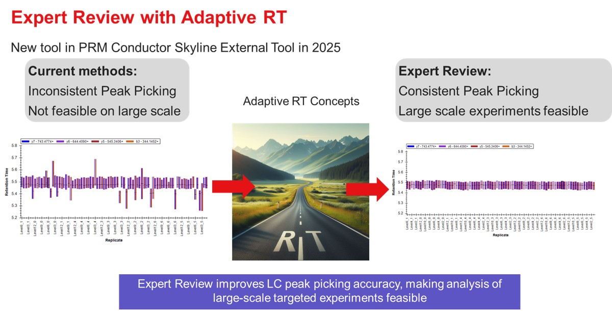
- To use Expert Review, you should have a reference set of data, where the all the peaks have been picked correctly. If you are doing a label-free experiment, the easiest way to obtain a reference file is to have a set of discovery data with compound IDs in it, ensuring that the correct peak was initially selected in Skyline. If the experiment you are doing uses heavy standards, then the reference data can come from injections of the neat standards.
- Expert Review utilizes two levels of analysis, a Replicate-level scoring based on an analysis of each replicate in isolation, and an Experiment-level re-scoring for each precursor, that considers all of its replicates.
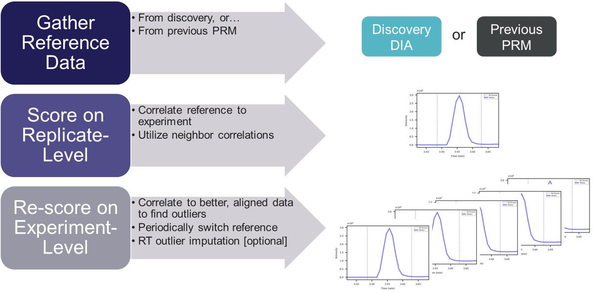
Expert review has mostly been used for analysis of dilution curves, which are challenging test cases for integration boundary determination, because by design there are many replicates where the analytes of interest are diluted to below limits of detection. We have found via manual inspection in many cases that Expert Review makes no errors, and those errors that do happen are typically either very small, or caused by the use of the RT outlier correction, which is not suitable for abrupt RT changes, and is an option that can be turned off.
Absolute Quantitation - PQ500
Absolute Quantitation - PQ500
For this walkthrough, we will use data from our paper on Stellar MS with Adaptive RT and PRM Conductor. This section uses a dilution of the Biognosys PQ500 sample in plasma.
- Obtain the Skyline data files in this Panorama repo, in the Raw Data \ Expert Review folder. Open the Skyline file Absolute Quantitation \ 60spd_dilution_lightheavy_skyline.sky.
For me, the document opened with the NLVVIPK peptide selected, illustrating one of the great challenges of performing dilution curves with samples like the PQ500. You can use Ctrl+F and search for this peptide sequence, or peruse the document ande find many other such examples. Many of the targets, like this one, don't have appreciable endogenous signal, therefore peptides like this one will be problematic to analyze if the Skyline document is set to Settings / Peptide Settings / Modification Settings / Internal Standard Type / Light. Of course there are some peptides. like LVTDLTK from Albumen, that have enormous endogenous signal, and for which there is no issue using the Light Internal Standard Type for a dilution curve. If the Internal Standard Type is set to Heavy, there traditionally were problems when the dilutions are low enough that there is little to no Heavy standard signal, and the boundaries would get set more or less randomly. Expert Review aims to fix this problem.
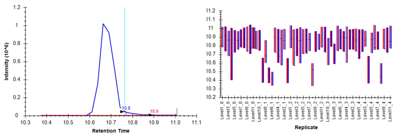
Expert Review - Light Boundary Mode
First we will look at the Expert Review results with the light Isotope boundary type, to illustrate the potential pitfalls of this mode for large assays that don't have much endogenous signal for many targets. Launch Expert Review after having installed or upgraded your PRM Conductor instance, by running Tools / Thermo / Expert Review. You will see the green progress bar move as Skyline exports the data set, and finally Expert Review will open. If this is the first time that you've run Expert Review, the Reference Grid will look like below, where the replicates for this experiment are listed. The replicates are listed from first-acquired to last-acquired, and the first replicate has a checkbox next to it.
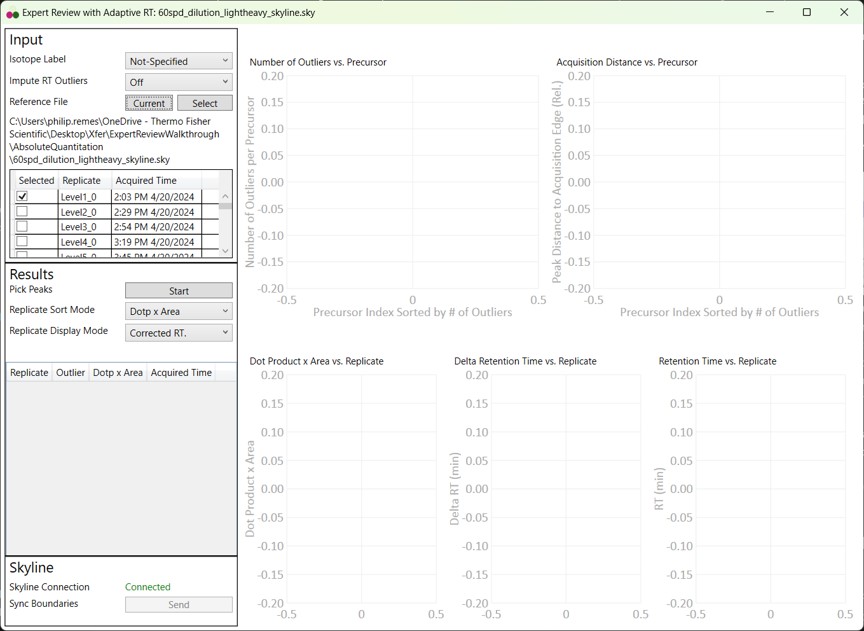
- If you select the checkbox, the grid will be highlighted in red, and you can't press the Results:Start button. We always need to have at least one reference replicate selected.
- If you are using a replicate from the same Skyline file you are using for analysis, and it isn't the first-acquired replicate, you'll have deselect the first replicate, find the replicate you want, and select it.
- I like to save the reference replicate in another separate Skyline file and press Select to open a file-chooser, and select that file.
- Expert Review remembers the last reference file that you used, which is someties convenient, but sometimes annoying when you switch experiments and forget to change the reference, and then there will be errors when your reference precursors don't include your experiment precursors.
- Press the Select button, and choose the other Skyline file in the Absolute Quantitation folder, P1_Neo_60SPD_HeavyLight_Reference.sky. This file has the last replicate from a test of the measurement precision of the assay.
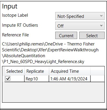
- For the first test, select Isotope Label Light. When Isotope Label is set to Light or Heavy, a new option appears, Use Other Label's Info. This allows to use the data from the other isotope label, in this case the heavy data, to ensure a more consistent integration boundary position. Usually this is a good idea. There could be some case where the other isotope label data are not very constant, which is why there is an option to turn this off, but it defaults to On.
- I usually set Impute RT Outliers to On, if there is a smoothly varying trend of RT with acquisition time, or no RT drift, as this option could help the peak picking accuracy, by on the order of tenths of a percent. However there have been cases where experiments have some sharp change in retention time between replicates, where this option doesn't work as well as you might want it to.
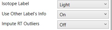
- Press the Start button and the processing starts. On my laptop, it takes 1 minute to process the data for these 804 light/heavy precursors and 55 replicates.
- Note that we have not pressed the Send button yet, so Skyline still has its original integration boundaries.
- When the processing finishes, Expert Review ranks the peptides according to how many adjustments were made on the Experiment-level. This is a general measure of how big of a challenge the data posed. Right now, the first, or worst quality precursor is selected when the processing is finished.
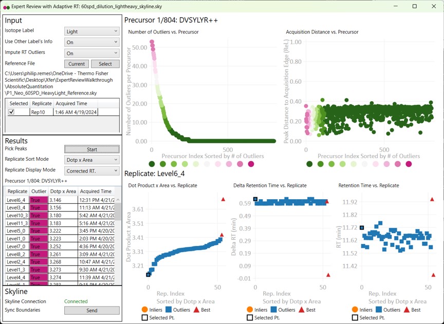
- Skyline is synced to Expert Review in a one-way mode, such that the active precursor in Expert Review is made active in Skyline, but not vice-versa.
- Switch to the Skyline document to see the chromatograms for DVSYLYR, the one that has the most outliers. This is a challenging one for the light mode, because there is a huge endogenous peak at a retention time that is nearby to the heavy standard.
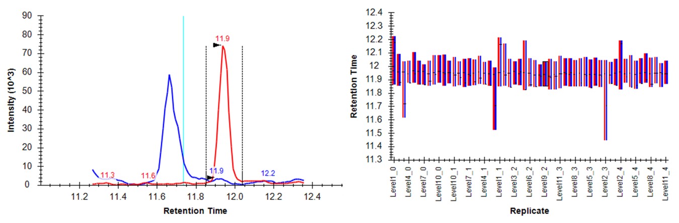
- Either press the Right key 3 times, or try to click the mouse on the 4th dot on the Number of Outliers vs Precursor graph. You can also zoom in on the plot with the mouse wheel, and double click to unzoom. You'll have highlighted the LTPTLYVGK precursor. This one has an endogenous time profile that is variable and does not present a clear pattern. It's no wonder that Skyline had a hard time here, using light boundaries.
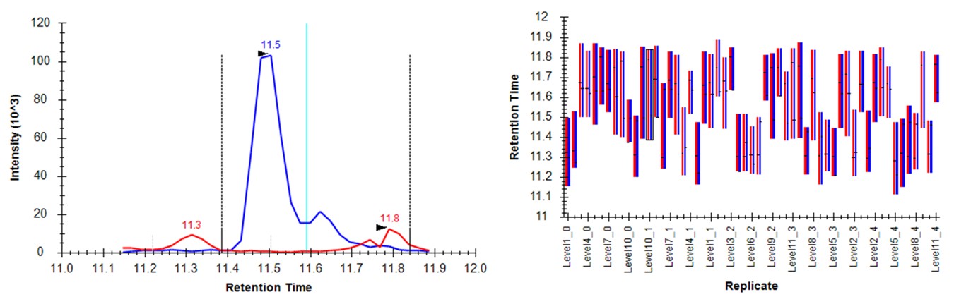
- Press the Send button. Skyline will take a few moments to import the Expert Review boundaries, and will stay on the LTPTLYVGK peptide. Now the boundaries are certainly more consistent, but they are in the wrong place, because the light data don't have a very good peak in the neighborhood of the actual heavy standard peak. The areas of the heavy peptides don't match with the expected dilution trend. This example shows again the perils of using light boundaries when there is no good light reference peak. If you go back to the DVSYLYR peptide, you'll see that here the results are not so satifactory either. In any event, Expert Review let us know which precursors were the most problematic. If you peruse the precursors that had fewer outliers corrected, the results are excellent. Let's see how things improve when we use the heavy peak boundaries.
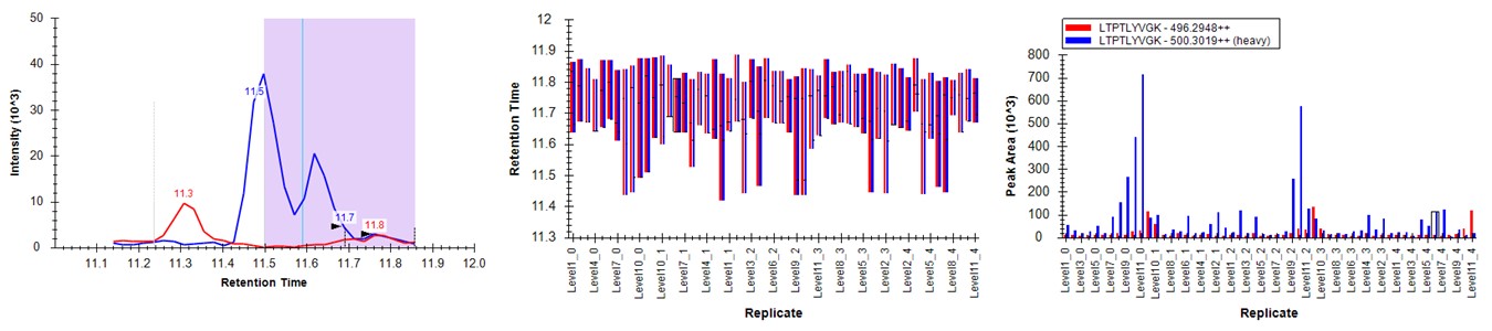
Expert Review - Heavy Boundary Mode
- Select Isotope Label Heavy, and Press the Start button. When the processing finishes, press the Send button. Notice that now the outliers plot shows that most precursors have many more replicates that needed Experiment-level correction. This makes sense, because every precursor is getting diluted below its limit of detection, eventually, and its replicate data no longer matches the reference.
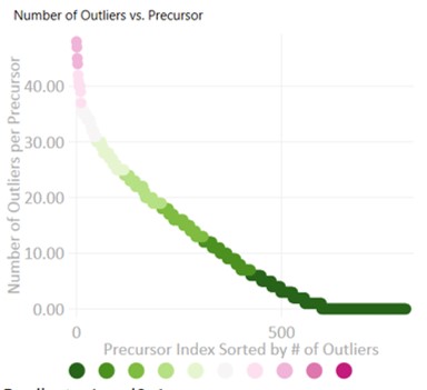
- Peruse the data a little bit, pressing the Right key on Expert review to look at the most challenging cases. They look good! In some cases, there are early eluting peaks with variable peaks that give poor results, or very nearby interferences that affect the absolute peak areas. There could be some improvements to be made in terms of making the integration boundary widths more consistent.
- If we look at the LTPTLYVGK example from before, the low level interference does move the boundary a little bit, but the areas of the peaks are much more in line with the dilution curve.
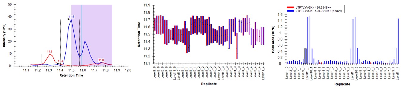
Conclusion
When performing dilutions of heavy standards in an endogenous background, use the heavy boundary mode, unless you are sure that all or most of the peptides have appreciable endogenous signal to use as references.
Label Free - E. Coli
Label Free - E. Coli
For this walkthrough, we will continue using data from our paper on Stellar MS with Adaptive RT and PRM Conductor. This section uses a dilution of E. Coli in a HeLa background.
- Open the file LabelFree / ecoli_small_dilution_skyline.sky.
- If you haven't installed the new PRM Conductor v1.1, do that
- Run Expert Review
- If you just did the absolute quantitation walkthrough, then Expert Review has the reference for that experiment, and is set to Isotope Label Heavy. We have to update this.
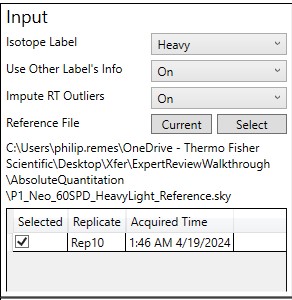
- Set Isotope Label to Not-Specified
- Press the Current Button. The reference grid is populated now with the replicates from this dilution. You could choose a replicate from this experiment to use as a reference, but I find it more convenient to use a separate reference.
- In the label free scenario, we have the advantage that we likely imported search results into Skyline, so all of the peaks likely are chosen correctly in some initial data set. The only problem is that the quality of these data may be low, due to the low injection times often used for a discovery DIA experiment.
- What I do is use the GPF as a reference to pick the peaks in PRM validation experiments, and then eventually use a PRM experiment as the reference for the remaining experiments in a study.
- Press the Select button, and choose LabelFree / ecolihela_gpf.sky. There are 6 LC injections that comprise this data set, but they were imported as a multi-injection replicate to Skyline, so they show up as a single replicate here. If you had imported the data as 6 single replicates, you could select all 6 of them in the reference grid here.
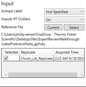
- Press Start to process the data, and then press the Send button to send the integration boundaries to Skyline.
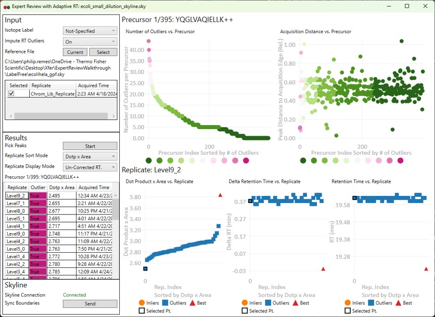
- Have a look at the worst precursors using the Right key. There are a few that should never have been included in the assay. Let's look at the worst precursor according to the number of outliers, YQGLVAQIELLK. Most of the integration boundaries are over near a small peak at the boundary. If we open the GPF Skyline document and find this peptide, we'll see that it has many more transitions.
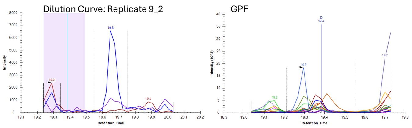
- Let's see if we can get better results by using a better reference, from PRM data. Press Select and choose the file ecoli_small_reference.sky, press Start, and then Send when the processing finishes. Use Ctrl+F and paste in YQGLVAQIELLK and search for it. Now these data look very nice, because the reference and dilution experiment data are very similar.
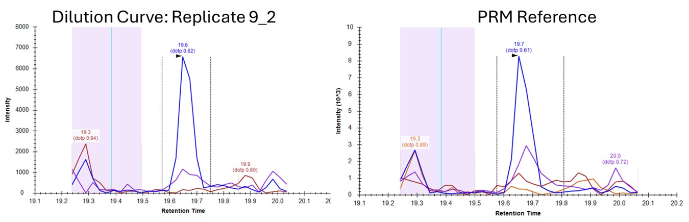
If you look in the Skyline Immediate Window log, you'll see some messages of the type:
2025-05-20 10:22:15.7649|WARN|Thermo.TNG.PeakPick.Algorithm.Logger|No reference found for precursor Sequence: QIIIATGEGAK
If you go to the reference file, for some reason this peptide is not found. It looks like there was an acquisition issue with this one, potentially caused by narrow acquisition windows, and an issue with Adaptive RT having a jump in its estimated retention time. We have since done some work to mitigate this kind of occurance in 1.1, so we hope that the low rate of such occurence will be even lower now.
- Now if we press the Right and Left keys in Expert Review to look through the precursors with the most outliers, they look good. There are a few precursors that we would consider dropping from the assay, or at least from the Skyline file, due to low S/N or bad peak shapes, but the peak integration boundaries look nice.
Conclusion
Expert Review can work with label free data too, but the similarity of the reference data to the later experiments is important. Another thing that we could have done to improve the results using the GPF reference, is to use PRM Conductor on it that file, and then make sure that the experiment data use the same transitions as the reference. That would have been what one normally would do, but these data were used to demonstrate the point. Since Stellar is a PRM machine, using the new transitions would just be a matter of reimporting the raw files in the Skyline documents.